Thursday 13 October 2022

Relational Properties of DE-9IM spatial predicates

There is an elegant mathematical theory of binary relations.  Homogeneous relations are an important subclass of binary relations in which both domains are the same.  A homogeneous relation R is a subset of all ordered pairs (x,y) with x and y elements of the domain.  This can be thought of as a boolean-valued function R(x,y), which is true if the pair has the relationship and false if not.

The restricted structure of homogeneous relations allows describing them by various properties, including:

Reflexive - R(x, x) is always true

Irreflexive - R(x, x) is never true

Symmetric - if R(x, y), then R(y, x)

Antisymmetric - if R(x, y) and R(y, x), then x = y

Transitive - if R(x, y) and R(y, z), then R(x, z)

The Dimensionally Extended 9-Intersection Model (DE-9IM) represents the topological relationship between two geometries.  

Various useful subsets of spatial relationships are specified by named spatial predicates.  These are the basis for spatial querying in many spatial systems including the JTS Topology Suite, GEOS and PostGIS.

The spatial predicates are homogeneous binary relations over the Geometry domain  They can thus be categorized in terms of the relational properties above.  The following table shows the properties of the standard predicates:

PredicateReflexive /
Irreflexive
Symmetric /
Antisymmetric
Transitive

EqualsRST
IntersectsRS-
DisjointRS-
ContainsRA-
WithinRA-
CoversRAT
CoveredByRAT
CrossesIS-
OverlapsIS-
TouchesIS-

Notes

  • Contains and Within are not Transitive because of the quirk that "Polygons do not contain their Boundary" (explained in this post).  A counterexample is a Polygon that contains a LineString lying in its boundary and interior, with the LineString containing a Point that lies in the Polygon boundary.  The Polygon does not contain the Point.  So Contains(poly, line) = true and Contains(line, pt) = true, but Contains(poly, pt) = false.   The predicates Covers and CoveredBy do not have this idiosyncrasy, and thus are transitive.

Wednesday 24 August 2022

Validating Polygonal Coverages in JTS

The previous post discussed polygonal coverages and outlined the plan to support them in the JTS Topology Suite.  This post presents the first step of the plan: algorithms to validate polygonal coverages.  This capability is essential, since coverage algorithms rely on valid input to provide correct results.  And as will be seen below, coverage validity is usually not obvious, and cannot be taken for granted.  

As described previously, a polygonal coverage is a set of polygons which fulfils a specific set of geometric conditions.  Specifically, a set of polygons is coverage-valid if and only if it satisfies the following conditions:

  • Non-Overlapping - polygon interiors do not intersect
  • Edge-Matched (also called Vector-Clean and Fully-Noded) - the shared boundaries of adjacent polygons has the same set of vertices in both polygons
The Non-Overlapping condition ensures that no point is covered by more than one polygon.  The Edge-Matched condition ensures that coverage topology is stable under transformations such as reprojection, simplification and precision reduction (since even if vertices are coincident with a line segment in the original dataset, this is very unlikely to be the case when the data is transformed).  
An invalid coverage which violates both (L) Non-Overlapping and (R) Edge-Matched conditions (note the different vertices in the shared boundary of the right-hand pair)

Note that these rules allow a polygonal coverage to cover disjoint areas.  They also allow internal gaps to occur between polygons.  Gaps may be intentional holes, or unwanted narrow gaps caused by mismatched boundaries of otherwise adjacent polygons.  The difference is purely one of size.  In the same way, unwanted narrow "gores" may occur in valid coverages.  Detecting undesirable gaps and gores will be discussed further in a subsequent post. 

Computing Coverage Validation

Coverage validity is a global property of a set of polygons, but it can be evaluated in a local and piecewise fashion.  To confirm a coverage is valid, it is sufficient to check every polygon against each adjacent (intersecting) polygon to determine if any of the following invalid situations occur:
  • Interiors Overlap:
    • the polygon linework crosses the boundary of the adjacent polygon
    • a polygon vertex lies within the adjacent polygon
    • the polygon is a duplicate of the adjacent polygon
  • Edges do not Match:
    • two segments in the boundaries of the polygons intersect and are collinear, but are not equal 
If neither of these situations are present, then the target polygon is coverage-valid with respect to the adjacent polygon.  If all polygons are coverage-valid against every adjacent polygon then the coverage as a whole is valid.

For a given polygon it is more efficient to check all adjacent polygons together, since this allows faster checking of valid polygon boundary segments.  When validation is used on datasets which are already clean, or mostly so, this improves the overall performance of the algorithm.  

Evaluating coverage validity in a piecewise way allows the validation process to be parallelized easily, and executed incrementally if required.

JTS Coverage Validation

Validation of a single coverage polygon is provided by the JTS CoveragePolygonValidator class.  If a polygon is coverage-invalid due to one or more of the above situations, the class computes the portion(s) of the polygon boundary which cause the failure(s).  This allows the locations and number of invalidities to be determined and visualized.

The class CoverageValidator computes coverage-validity for an entire set of polygons.  It reports the invalid locations for all polygons which are not coverage-valid (if any). 

Using spatial indexing makes checking coverage validity quite performant.  For example, a coverage containing 91,384 polygons with 10,474,336 vertices took only 6.4 seconds to validate.  In this case the coverage is nearly valid, since only one invalid polygon was found. The invalid boundary linework returned by CoverageValidator allows easily visualizing the location of the issue.

A polygonal dataset of 91,384 polygons, containing a single coverage-invalid polygon

The invalid polygon is a tiny sliver, with a single vertex lying a very small distance inside an adjacent polygon.  The discrepancy is only visible using the JTS TestBuilder Reveal Topology mode.

The size of the discrepancy is very small.  The vertex causing the overlap is only 0.0000000001 units away from being valid:

[921]  POLYGON(632)
[922:4]  POLYGON(5)
Ring-CW  Vert[921:0 514]  POINT ( 960703.3910000008 884733.1892000008 )
Ring-CW  Vert[922:4:0 3]  POINT ( 960703.3910000008 884733.1893000007 )

This illustrates the importance of having fast, robust automated validity checking for polygonal coverages, and providing information about the exact location of errors.

Real-world testing

With coverage validation now available in JTS, it's interesting to apply it to publicly available datasets which (should) have coverage topology.  It is surprising how many contain validity errors.  Here are a few examples:

SourceCity of Vancouver
DatasetZoning Districts


This dataset contains 1,498 polygons with 57,632 vertices. There are 379 errors identified, which mainly consist of very small discrepancies between vertices of adjacent polygons.
Example of a discrepant vertex in a polygon


SourceBritish Ordnance Survey OpenData
DatasetBoundary-Line
Fileunitary_electoral_division_region.shp


This dataset contains 1,178 polygons with 2,174,787 vertices. There are 51 errors identified, which mainly consist of slight discrepancies between vertices of adjacent polygons. (Note that this does not include gaps, which are not detected by CoverageValidator.  There are about 100 gaps in the dataset as well.)
An example of overlapping polygons in the Electoral Division dataset


SourceHamburg Open Data Platform
DatasetVerwaltungsEinheit (Administrative Units)


The dataset (slightly reduced) contains 7 polygons with 18,254 vertices.  Coverage validation produces 64 error locations.  The errors are generally small vertex discrepancies producing overlaps.  Gaps exist as well, but are not detected by the default CoverageValidator usage.
An example of overlapping polygons (and a gap) in the VerwaltungsEinheit dataset


As always, this code will be ported to GEOS.  A further goal is to provide this capability in PostGIS, since there are likely many datasets which could benefit from this checking.  The piecewise implementation of the algorithm should mesh well with the nature of SQL query execution.

And of course the next logical step is to provide the ability to fix errors detected by coverage validation.   This is a research project for the near term.

UPDATE: my colleague Paul Ramsey pointed out that he has already ported this code to GEOS.  Now for some performance testing!

Sunday 24 July 2022

Polygonal Coverages and Operations in JTS

An important concept in spatial data modelling is that of a coverage.  A coverage models a two-dimensional region in which every point has a value out of a range (which may be defined over one or a set of attributes).  Coverages can be represented in both of the main physical spatial data models: raster and vector.  In the raster data model a coverage is represented by a grid of cells with varying values.  In the vector data model a coverage is a set of non-overlapping polygons (which usually, but not always, cover a contiguous area).  

This post is about the vector data coverage model, which is termed (naturally) a polygonal coverage. These are used to model regions which are occupied by discrete sub-regions with varying sets of attribute values.  The sub-regions are modelled by simple polygons.  The coverage may contain gaps between polygons, and may cover multiple disjoint areas.  The essential characteristics are:

  • polygon interiors do not overlap
  • the common boundary of adjacent polygons has the same set of vertices in both polygons.

There are many types of data which are naturally modelled by polygonal coverages.  Classic examples include:

  • Man-made boundaries
    • parcel fabrics
    • political jurisdictions
  • Natural boundaries
    • vegetation cover
    • land use
A polygonal coverage of regions of France

Topological and Discrete Polygonal Coverages


There are two ways to represent polygonal coverages: as a topological data structure, or as a set of discrete polygons.  
A coverage topology consists of linked faces, edges and nodes. The edges between two nodes form the shared boundary between two faces.  The coverage polygons can be reconstituted from the edges delimiting each face.  
The discrete polygon representation is simpler, and aligns better with the OGC Simple Features model.  It is simply a collection of polygons which satisfy the coverage validity criteria given above.
Most common spatial data formats support only a discrete polygon model, and many coverage datasets are provided in this form.  However, the lack of inherent topology means that datasets must be carefully constructed to ensure they have valid coverage topology.  In fact, many available datasets contain coverage invalidities.  A current focus of JTS development is to provide algorithms to detect this situation and provide the locations where the polygons fail to form a valid coverage.

Polygonal Coverage Operations

Operations which can be performed on polygonal coverages include:

  • Validation - check that a set of discrete polygons forms a valid coverage
  • Gap Detection - check if a polygonal coverage contains narrow gaps (using a given distance tolerance)
  • Cleaning - fix errors such as gaps, overlaps and slivers in a polygonal dataset to ensure that it forms a clean, valid coverage
  • Simplification - simplify (generalize) polygon boundary linework, ensuring coverage topology is preserved
  • Precision Reduction - reduce precision of polygon coordinates, ensuring coverage topology is preserved
  • Union - merge all or portions of the coverage polygons into a single polygon (or multipolygon, if the input contains disjoint regions)
  • Overlay - compute the intersection of two coverages, producing a coverage of resultant polygons 

Implementing polygonal coverage operations is a current focus for development in the JTS Topology Suite.  Since most operations require a valid coverage as input, the first goal is to provide Coverage Validation.  Cleaning and Simplification are priority targets as well.  Coverage Union is already available, as is Overlay (in a slightly sub-optimal way).  In addition,  a Topology data structure will be provided to support the edge-node representation.  (Yes, the Topology Suite will provide topology at last!).  Stay tuned for further blog posts as functionality is rolled out.

As usual, the coverage algorithms developed in JTS will be ported to GEOS, and will thus be available to downstream projects like PostGIS.

Tuesday 21 June 2022

JTS 1.19 Released

JTS 1.19 has just been released!  There is a great deal of new, improved and fixed functionality in this release - see the GitHub release page or the Version History for full details.

This blog has several posts describing new functionality in JTS 1.19:

New Functionality

Improvements


Many of these improvements have been ported to GEOS, and will appear in the soon-to-appear version 3.11.  In turn this has provided the basis for new and enhanced functions in the next PostGIS release, and will likely be available in other platforms via the many GEOS bindings and applications.

Monday 30 May 2022

Algorithm for Concave Hull of Polygons

The previous post introduced the new ConcaveHullOfPolygons class in the JTS Topology Suite.  This allows computing a concave hull which is constrained by a set of polygonal geometries.  This supports use cases including:

  • generalization of groups of polygon
  • joining polygons
  • filling gaps between polygons

A concave hull of complex polygons

The algorithm developed for ConcaveHullOfPolygons is a novel one (as far as I know).  It uses several features recently developed for JTS, including a neat trick for constrained triangulation.  This post describes the algorithm in detail.

The construction of a concave hull for a set of polygons uses the same approach as the existing JTS ConcaveHull implementation.  The space to be filled by a concave hull is triangulated with a Delaunay triangulation.  Triangles are then "eroded" from the outside of the triangulation, until a criteria for termination is achieved.  A useful termination criteria is that of maximum outside edge length, specified as either an absolute length or a fraction of the range of edge lengths.

For a concave hull of points, the underlying triangulation is easily obtained via the Delaunay Triangulation of the point set.  However, for a concave hull of polygons the triangulation required is for the space between the constraint polygons.  A simple Delaunay triangulation of the polygon vertices will not suffice, because the triangulation may not respect the edges of the polygons.  

Delaunay Triangulation of polygon vertices crosses polygon edges

What is needed is a Constrained Delaunay Triangulation, with the edge segments of the polygons as constraints (i.e. the polygon edge segments are present as triangle edges, which ensures that other edges in the triangulation do not cross them).  There are several algorithms for Constrained Delaunay Triangulations - but a simpler alternative presented itself.  JTS recently added an algorithm for computing Delaunay Triangulations for polygons.  This algorithm supports triangulating polygons with holes (via hole joining).  So to generate a triangulation of the space between the input polygons, they can be inserted as holes in a larger "frame" polygon.  This can be triangulated, and then the frame triangles removed. Given a sufficiently large frame, this leaves the triangulation of the "fill" space between the polygons, out to their convex hull. 

Triangulation of frame with polygons as holes

The triangulation can then be eroded using similar logic to the non-constrained Concave Hull algorithm.  The implementations all use the JTS Tri data structure, so it is easy and efficient to share the triangulation model between them. 

Triangulation after removing frame and eroding triangles

The triangles that remain after erosion can be combined with the input polygons to provide the result concave hull.  The triangulation and the input polygons form a polygonal coverage, so the union can be computed very efficiently using the JTS CoverageUnion class.  If required, the fill area alone can be returned as a result, simply by omitting the input polygons from the union.

Concave Hull and Concave Fill

A useful option is to compute a "tight" concave hull to the outer boundary of the input polygons.  This is easily accomplished by removing triangles which touch only a single polygon.  

Concave Hull tight to outer edges


Concave Hull of complex polygons, tight to outer edges.

Like the Concave Hull of Points algorithm, holes are easily supported by allowing erosion of interior triangles.

Concave Hull of Polygons, allowing holes

The algorithm performance is determined by the cost of the initial polygon triangulation.  This is quite efficient, so the overall performance is very good.

As mentioned, this seems to be a new approach to this geometric problem.  The only comparable implementation I have found is the ArcGIS tool called Aggregate Polygons, which appears to provide similar functionality (including producing a tight outer boundary).  But of course algorithm details are not published and the code is not available.  It's much better to have an open source implementation, so it can be used in spatial tools like PostGIS, Shapely and QGIS (based on the port to GEOS).  Also, this provides the ability to add options and enhanced functionality for use cases which may emerge once this gets some real-world use.

Friday 20 May 2022

Concave Hulls of Polygons

A common spatial need is to compute a polygon which contains another set of polygons.  There are numerous use cases for this; for example:

  • Generalizing groups of building outlines (questions: 1, 2
  • Creating "district" polygons around block polygons (questions: 1)
  • Removing gaps between sets of polygons (questions: 1, 2, 3, 4)
  • Joining two polygons by filling the space between them (questions: 1, 2)     
This post describes a new approach for solving these problems, via an algorithm for computing a concave hull with polygonal constraints.  The algorithm builds on recent work on polygon triangulation in JTS, and uses a neat trick which I'll describe in a subsequent post.  

Approach: Convex Hull

The simplest way to compute an area enclosing a set of geometries is to compute their convex hull.  But the convex hull is a fairly coarse approximation of the area occupied by the polygons, and in most cases a better representation is required.  

Here's an example of gap removal between two polygons.  Obviously, the convex hull does not provide anything close to the desired result: 

Approach: Buffer and Unbuffer

A popular suggestion is to buffer the polygon set by a distance sufficient to "bridge the gaps", and then "un-buffer" the result inwards by the same (negative) distance.  But the buffer computation can "round off" corners, which usually produces a poor match to the input polygons.  It also fills in the outer boundary of the original polygons.

Approach: Concave Hull of Points

A more sophisticated approach is to use a concave hull algorithm.  But most (or all?) available concave hull algorithms use points as the input constraints. The vertices of the polygons could be used as the constraint points, but since the polygon boundaries are not respected, the computed hull may cross the polygon edges and hence not cover the polygons.  

Densifying the polygon boundaries helps, but introduces another problem - the computed hull can extend beyond the outer boundaries of individual polygons.  And it introduces new vertices not present in the original data.

Solution: Concave Hull of Polygons

What is needed is a concave hull algorithm that accepts polygons as constraints, and thus respects their boundaries.  The JTS Topology Suite now provides this capability in a class called ConcaveHullOfPolygons (not a cute name, but descriptive).  It provides exactly the solution desired for the gap removal example:  

The Concave Hull of Polygons API

Like concave hulls of point sets, concave hulls of polygons form a sequence of hulls, with the amount of concaveness determined by a numeric parameter. ConcaveHullOfPolygons uses the same parameters as the JTS ConcaveHull algorithm.  The control parameter determines the maximum line length in the triangulation underlying the hull.  This can be specified as an absolute length, or as a ratio between the longest and shortest lines.  

Further options are:

  • The computed hull can be kept "tight" to the outer boundaries of the individual polygons.  This allows filling gaps between polygons without distorting their original outer boundaries.  Otherwise, the concaveness of the outer boundary will be decreased to match the distance parameter specified (which may be desirable in some situations).
  • Holes can be allowed to be present in the computed hull
  • Instead of the hull, the fill area between the input polygons can be computed.  
As usual, this code will be ported to GEOS, and from there it can be exposed in the downstream libraries and projects.

Examples of Concave Hulls of Polygons

Here are examples of using ConcaveHullOfPolygons for the use cases above:

Example: Generalizing Building Groups

Using the "tight" option allows following the outer building outlines.


Example: Aggregating Block Polygons

The concave hull of a set of block polygons for an oceanside suburb.  Note how the "tight" option allows the hull to follow the convoluted, fine-grained coastline on the right side.

Example: Removing Gaps to Merge Polygons

Polygons separated by a narrow gap can be merged by computing their concave hull using a small distance and keeping the boundary tight.

Example: Fill Area Between Polygons

The "fill area" portion of the hull between two polygons can be computed as a separate polygon. This could be used to provide an "Extend to Meet" construction by unioning the fill polygon with one of the input polygons.  It can also be used to determine the "visible boundary", provided by the intersection of the fill polygon with the input polygon(s).


Wednesday 4 May 2022

Using Outer Hulls for Smoothing Vectorized Polygons

The electrons were hardly dry on the JTS Outer and Inner Polygon Hull post when another interesting use case popped up on GIS StackExchange.  The question was how to remove aliasing artifacts (AKA "jaggies") from polygons created by vectorizing raster data, with the condition that the result should contain the original polygon.  

A polygon for Vancouver Island vectorized from a coarse raster dataset.  Aliasing artifacts are obvious.

This problem is often handled by applying a simplification or smoothing process to the "jaggy" polygon boundary.  This works, as long as the process preserves polygonal topology (e.g. such as the JTS TopologyPreservingSimplifier). But generally this output of this process does not contain the input polygon, since the simplification/smoothing can alter the boundary inwards as well as outwards.  

Simplification using TopologyPreservingSimplifier with distance = 0.1.  Artifacts are removed, but the simplified polygon does not fully contain the original.

In contrast, the JTS Polygon Outer Hull algorithm is designed to do exactly what is required: it reduces the number of vertices, while guaranteeing that the input polygon is contained in the result.  It is essentially a simplification method which also preserves polygonal topology (using an area-based approach similar to the Visvalingham-Whyatt algorithm).

Outer Hull using vertex ratio = 0.25.  Artifacts are removed, and the original polygon is contained in the hull polygon.

Here's a real-world example, taken from the GADM dataset for administrative areas of Germany.  The coastline of the state of Mecklenburg-Vorpommern appears to have been derived from a raster, and thus exhibits aliasing artifacts.  Computing the outer hull with a fairly conservative parameter eliminates most of the artifacts, and ensures polygonal topology is preserved.

A portion of the coastline of Mecklenburg-Vorpommern showing aliasing artifacts.  The Outer Hull computed with vertex ratio = 0.25 eliminates most artifacts, and preserves the coastline topology.

Future Work

A potential issue for using Outer Hull as a smoothing technique is the choice of parameter value controlling the amount of change.  The algorithm provides two options: the ratio of reduction in the number of vertices, or the fraction of change in area allowed.  Both of these are scale-independent, and reflect natural goals for controlling simplification.  But neither relate directly to the goal of removing "stairstep" artifacts along the boundary.  This might be better specified via a distance-based parameter. The parameter value could then be determined based on the known artifact size (i.e. the resolution of the underlying grid).  Since the algorithm for Outer Hull is quite flexible, this should be feasible to implement. 

Monday 25 April 2022

Outer and Inner Polygon Hulls in JTS

The JTS Topology Suite recently gained the ability to compute concave hulls.  The Concave Hull algorithm computes a polygon enclosing a set of points using a parameter to determine the "tightness".  However, for polygonal inputs the computed concave hull is built only using the polygon vertices, and so does not always respect the polygon boundaries.  This means the concave hull may not contain the input polygon.

It would be useful to be able to compute the "outer hull" of a polygon.  This is a valid polygon formed by a subset of the vertices of the input polygon which fully contains the input polygon.  Vertices can be eliminated as long as the resulting boundary does not self-intersect, and does not cross into the original polygon.

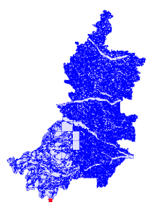
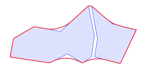
An outer hull of a polygon representing Switzerland

As with point-set concave hulls, the vertex reduction is controlled by a numeric parameter. This creates a sequence of hulls of increasingly larger area with smaller vertex counts.  At an extreme value of the parameter, the outer hull is the same as the convex hull of the input.
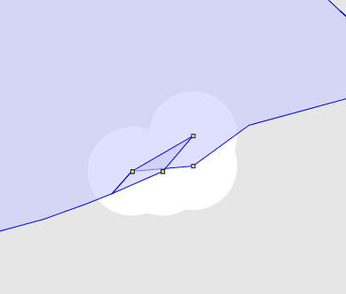
A sequence of outer hulls of New Zealand's North Island

The outer hull concept extends to handle holes and MultiPolygons.  In all cases the hull boundaries are constructed so that they do not cross each other, thus ensuring the validity of the result.

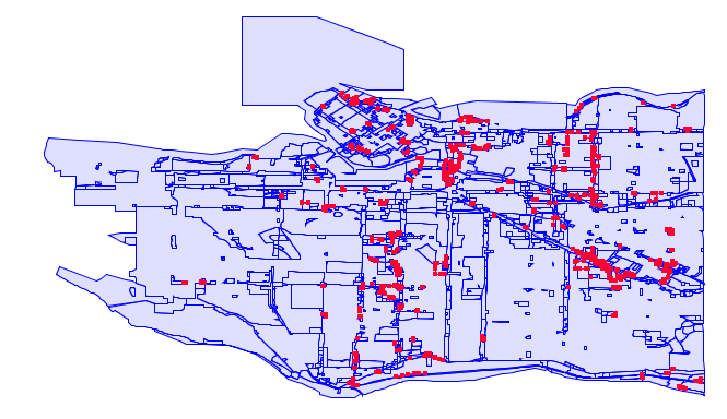
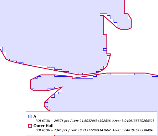
An outer hull of a MultiPolygon for the coast of Denmark.  The hull polygons do not cross.

It's also possible to construct inner hulls of polygons, where the constructed hull is fully within the original polygon.

An inner hull of Switzerland

Inner hulls also support holes and MultiPolygons.  At an extreme value of the control parameter, holes become convex hulls, and a polygon shell reduces to a triangle (unless blocked by the presence of holes).

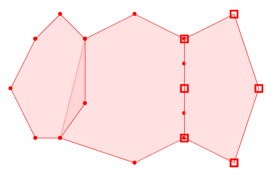
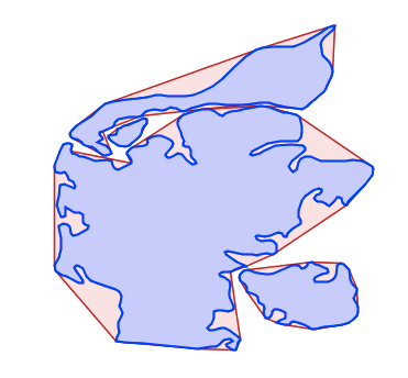
An inner hull of a lake with islands.  The island holes become convex hulls, and prevent the outer shell from reducing fully to a triangle

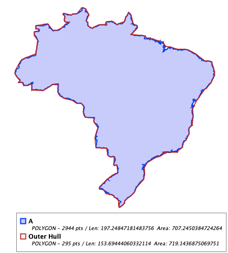
A hull can provide a significant reduction in the vertex size of a polygon for a minimal change in area. This could allow faster evaluation of spatial predicates, by pre-filtering with smaller hulls of polygons.

An outer hull of Brazil provides a 10x reduction in vertex size, with only ~1% change in area.

This has been on the JTS To-Do list for a while (I first proposed it back in 2009).  At that time it was presented as a way of simplifying polygonal geometry. Of course JTS has had the TopologyPreservingSimplifier for many years.  But it doesn't compute a strictly outer hull.  Also, it's based on Douglas-Peucker simplification, which isn't ideal for polygons.  

It seems there's quite a need for this functionality, as shown in these GIS-StackExchange posts (1, 2, 3, 4).  There's even existing implementations on Github: rdp-expansion-only and simplipy (both in Python) - but both of these sound like they have some significant issues. 

Recent JTS R&D (on concave hulls and polygon triangulation) has provided the basis for an effective, performant polygonal concave hull algorithm.  This is now released as the PolygonHullSimplifier class in JTS.

The PolygonHullSimplifier API

Polygon hulls have the following characteristics:

  • Hulls can be constructed for Polygons and MultiPolygons, including holes.
  • Hull geometries have the same structure as the input.  There is a one-to-one correspondence for  elements, shells and holes.
  • Hulls are valid polygonal geometries.
  • The hull vertices are a subset of the input vertices.

The PolygonHullSimplifier algorithm supports computing both outer and inner hulls. 

  • Outer hulls contain the input geometry.  Vertices forming concave corners (convex for holes) are removed.  The maximum outer hull is the convex hull(s) of the input polygon(s), with holes reduced to triangles.
  • Inner hulls are contained within the input geometry.  Vertices forming convex corners (concave for holes) are removed.   The minimum inner hull is a triangle contained in (each) polygon, with holes expanded to their convex hulls.  

The number of vertices removed is controlled by a numeric parameter.  Two different parameters are provided:

  • the Vertex Number Fraction specifies the desired result vertex count as a fraction of the number of input vertices.  The value 1 produces the original geometry.  Smaller values produce simpler hulls.  The value 0 produces the maximum outer or minimum inner hull.
  • the Area Delta Ratio specifies the desired maximum change in the ratio of the result area to the input area.  The value 0 produces the original geometry.  Larger values produce simpler hulls. 
Defining the parameters as ratios means they are independent of the size of the input geometry, and thus easier to specify for a range of inputs.  Both parameters are targets rather than absolutes; the validity constraint means the result hull may not attain the specified value in some cases. 

Algorithm Description

The algorithm removes vertices via "corner clipping".  Corners are triangles formed by three consecutive vertices in a (current) boundary ring of a polygon.  Corners are removed when they meet certain criteria.  For an outer hull, a corner can be removed if it is concave (for shell rings) or convex (for hole rings).  For an inner hull the removable corner orientations are reversed.  

In both variants, corners are removed only if the triangle they form does not contain other vertices of the (current) boundary rings.  This condition prevents self-intersections from occurring within or between rings. This ensures the resulting hull geometry is topologically valid.  Detecting triangle-vertex intersections is made performant by maintaining a spatial index on the vertices in the rings.  This is supported by an index structure called a VertexSequencePackedRtree.  This is a semi-static R-tree built on the list of vertices of each polygon boundary ring.  Vertex lists typically have a high degree of spatial coherency, so the constructed R-tree generally provides good space utilization.  It provides fast bounding-box search, and supports item removal (allowing the index to stay consistent as ring vertices are removed).

Corners that are candidates for removal are kept in a priority queue ordered by area.  Corners are removed in order of smallest area first.  This minimizes the amount of change for a given vertex count, and produces a better quality result.  Removing a corner may create new corners, which are inserted in the priority queue for processing.  Corners in the queue may be invalidated if one of the corner side vertices has previously been removed; invalid corners are discarded. 

This algorithm uses techniques originated for the Ear-Clipping approach used in the JTS PolgyonTriangulator implementation. It also has a similarity to the Visvalingham-Whyatt simplification algorithm.  But as far as I know using this approach for computing outer and inner hulls is novel. (After the fact I found a recent paper about a similar construction called a Shortcut Hull [Bonerath et al 2020], but it uses a different approach).

Further Work

It should be straightforward to use this same approach to implement a variant of Topology-Preserving Simplifier using the corner-area-removal approach (as in Visvalingham-Whyatt simplification).  The result would be a simplified, topologically-valid polygonal geometry.  The simplification parameter  limits the number of result vertices, or the net change in area.  The resulting shape would be a good approximation of the input, but is not necessarily be either wholly inside or outside.


Thursday 27 January 2022

Cubic Bezier Curves in JTS

As the title of this blog indicates, I'm a fan of linearity.  But sometimes a little non-linearity makes things more interesting.  A convenient way to generate non-linear curved lines is to use Bezier Curves.  Bezier Curves are curves defined by polynomials.  Bezier curves can be defined for polynomials of any degree, but a popular choice is to use cubic Bezier curves defined by polynomials of degree 3.  These are relatively easy to implement, visually pleasing, and versatile since they can model ogee or sigmoid ("S"-shaped) curves.

A single cubic Bezier curve is specified by four points: two endpoints forming the baseline, and two control points.  The curve shape lies within the quadrilateral convex hull of these points.

Note: the images in this post are created using the JTS TestBuilder.

Cubic Bezier Curves, showing endpoints and control points

A sequence of Bezier curves can be chained together to form a curved path of any required shape. There are several ways to join composite Bezier curves.  The simplest join constraint is C0-continuity: the curves touch at endpoints, but the join may be a sharp angle.  C1-continuity (differentiable) makes the join smooth. This requires the control vectors at a join point to be collinear and opposite.  If the control vectors are of different lengths there will be a different radius of curvature on either side.  The most visually appealing join is provided by C2-continuity (twice-differentiable), where the curvature is identical on both sides of the join.  To provide this the control vectors at a vertex must be collinear, opposite and have the same length.

Bezier Curve with C2-continuity

A recent addition to the JTS Topology Suite is the CubicBezierCurve class, which supports constructing Bezier Curves from LineStrings and Polygons.  JTS only supports representing linear geometries, so curves must be approximated by sequences of line segments. (The buffer algorithm uses this technique to approximate the circular arcs required by round joins.)   


Bezier Curve approximated by line segments

Bezier curves can be generated on both lines and polygons (including holes):
Bezier Curve on a polygon

There are two ways of specifying the control points needed to define the curve:  

Alpha (Curvedness) Parameter

The easiest way to define the shape of a curve is via the parameter alpha, which indicates the "curvedness".  This value is used to automatically generate the control points at each vertex of the baseline.  A value of 1 creates a roughly circular curve at right angles.  Higher values of alpha make the result more curved; lower values (down to 0) make the curve flatter.

Alpha is used to determine the length of the control vectors at each vertex.  The control vectors on either side of the vertex are collinear and of equal length, which provides C2-continuity.  The angle of the control vectors is perpendicular to the bisector of the vertex angle, to make the curve symmetrical.  

Bezier Curve for alpha = 1
Bezier Curve for alpha = 1.3

Bezier Curve for alpha = 0.3


Explicit Control Points

Alternatively, the Bezier curve control points can be provided explicitly.  This gives complete control over the shape of the generated curve.  Two control points are required for each line segment of the baseline geometry, in the same order.  A convenient way to provide these is as a LineString (or MultiLineString for composite geometries) containing the required number of vertices.


Bezier Curve defined by control points, with C2 continuity

When using this approach only C0-continuity is provided automatically.  The caller must enforce C1 or C2-continuity via suitable positioning of the control points.

Bezier Curve defined by control points showing C0 and C1 continuity

Further Ideas

  • Allow specifying the number of vertices used to approximate each curve
  • Add a function to return the constructed control vectors (e.g. for display and analysis purposes)
  • Make specifying explicit control points easier by generating C2-continuous control vectors from a single control point at each vertex

Tuesday 18 January 2022

Concave Hulls in JTS

A common spatial need is to find a polygon that accurately represents a set of points.  The convex hull of the points often does not provide this, since it can enclose large areas which contain no points.  What is required is a non-convex hull, often termed the concave hull.  

The Convex Hull and a Concave Hull of a point set

A concave hull is generally considered to have some or all of the following properties:

  • The hull is a simply connected polygon
  • It contains all the input points
  • The vertices in the hull polygon boundary are all input points
  • The hull may or may not contain holes
For a typical point set there are many polygons which meet these criteria, with varying degrees of concaveness.  Concave Hull algorithms provide a numeric parameter which controls the amount of concaveness in the result.  The nature of this parameter is particularly important, since it affects the ease-of-use in practical scenarios.  Ideally it has the following characteristics:

  • Simple geometric basis: this allows the user to understand the effect of the parameter and aids in determining an effective value
  • Scale-free (dimensionless): this allows a single parameter value to be effective on varying sizes of geometry, which is essential for batch or automated processing
  • Local (as opposed to global):  A local property (such as edge length) gives the algorithm latitude to determine the concave shape of the points. A global property (such as area) over-constrains the possible result. 
  • Monotonic area:  larger (or smaller) values produce a sequence of more concave areas
  • Monotonic containment :the sequence of hulls produced are topologically nested
  • Convex-bounded: an extremal value produces the convex hull

This is a well-studied problem, and many different approaches have been proposed.  Some notable ones are:

Of these, Delaunay Erosion (Chi-shapes) offers the best set of features.  It is straightforward to code and is performant.  It uses the control parameter of Edge Length Ratio, a fraction of the difference between the longest and shortest edges in the underlying Delaunay triangulation.  This is easy to reason about, since it is scale-free and corresponds to a simple property of the point set (that of distance between vertices).  It can be extended to support holes.  And it has a track record of use, notably in Oracle Spatial.  

ConcaveHull generated by Delaunay Erosion with Edge Length Ratio = 0.3

Recently the Park-Oh algorithm has become popular, thanks to a high-quality implementation in Concaveman project (which has spawned numerous ports).  However, it has some drawbacks.  It can't support holes (and likely not disconnected regions and discarding outlier points).  As the paper points out and experiment confirms, it produces rougher outlines than the Delaunay-based algorithm.  Finally, the control parameter for Delaunay Erosion has a simpler geometrical basis which makes it easier to use.

Given these considerations, the new JTS ConcaveHull algorithm utilizes Delaunay Erosion. The algorithm ensures that the computed hull is simply connected, and contains all the input points.  The Edge Length Ratio is used as the control parameter. A value of 1 produces the convex hull; 0 produces a concave hull of minimal size.  Alternatively the maximum edge length can be specified directly. This allows alternative strategies to determine an appropriate length value; for instance, another possibility is to use a fraction of the longest edge in the Minimum Spanning Tree of the input points.  

The recently-added Tri data structure provides a convenient basis for the implementation,.  It operates as follows:

  1. The Delaunay Triangulation of the input points is computed and represented as a set of of Tris
  2. The Tris on the border of the triangulation are inserted in a priority queue, sorted by longest boundary edge
  3. While the queue is non-empty, the head Tri is popped from the queue.  It is removed from the triangulation if it does not disconnect the area.  Insert new border Tris into the queue if they have a boundary edge length than the target length
  4. The Tris left in the triangulation form the area of the Concave Hull 

Thanks to the efficiency of the JTS Delaunay Triangulation the implementation is quite performant, approaching the performance of a Java port of Concaveman.  

Concave Hull of Ukraine dataset; Edge Length Ratio = 0.1

Optionally holes can be allowed to be present in the hull polygon (while maintaining a simply connected result).  A classic demonstration of this is to generate hulls for text font glyphs:


This algorithm is in the process of being ported to GEOS.  The intention is to use it to enhance the PostGIS ST_ConcaveHull function, which has known issues and has proven difficult to use.

Further Ideas

  • Disconnected Result - It is straightforward to extend the algorithm to allow a disconnected result (i.e. a MultiPolygon).  This could be provided as an option.
  • Outlier Points - It is also straightforward to support discarding "outlier" points.
  • Polygon Concave Hull - computing a concave "outer hull" for a polygon can be used to simplify the polygon while guaranteeing the hull contains the original polygon.  Additionally, an "inner hull" can be computed which is fully contained in the original.  The implementation of a Polygon Concave Hull algorithm is well under way and will be released in JTS soon.