Thursday, 21 November 2019

Variable-distance buffering in JTS

The operation of buffering a geometry is a core geospatial concept.  Standard buffers are computed using a fixed distance around the input geometry. JTS has provided a buffer implementation since its inception, and this is used in GEOS and all the other downstream projects as well. 

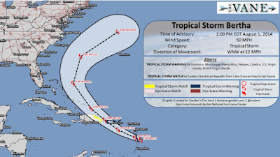
One way to generalize the buffer concept is to allow the buffer distance to vary along the geometry.  As often the case with geospatial concepts this construction has a few different names, including tapered buffer, cone buffer, varying buffer, and variable-distance buffer.  The classic use case for variable-distance buffers is generating polygons for the "cone of uncertainty" along predicted hurricane tracks:


Another use case is depicting rivers showing the width of reaches along the river course. 

I took a crack at prototyping "variable width buffers" a few years ago, in the JTS Lab.  Recently there were a couple of GIS StackExchange posts looking for this functionality in PostGIS and Shapely   They were good motivation to buff up the prototype and move it into JTS core.  But I was dismayed to realize that the output had some serious deficiencies, due to an overly-simplistic algorithm.  The idea in the Lab code was appealingly simple: compute buffer circles around each line vertex at the specified distance, and union (merge) them with trapezoids computed around the connecting line segment.  But this produced ugly discontinuities for large deltas in buffer distances. 

For such a seemingly simple concept there is surprisingly little prior art to be found.  Even the GIS That Shall Not Be Named does not seem to provide a native variable buffer function (although recently I found a couple of user contribs which do, to some extent).   There's an implementation in QGIS - but since it seems to be based on the original problematic JTS code that didn't really help.   So I had the fun of coding it up from scratch.  

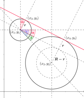
The problem with the original code is that it should have used the outer tangent lines to the buffer circles at each vertex.  Wikipedia has a good discussion of this construction.  Even better, it provides an elegant mathematical algorithm, which worked perfectly when coded up.


The construction computes a single tangent segment.  The opposite segment is simply the reflection in the line between the circle centres.  The geometric math to handle this is now provided for reuse as  LineSegment.reflect().  Finally, it is notoriously tricky to produce buffer curves with high quality in the fine details.  In this case, generating the line segment buffer caps required care to avoid creating out-of-phase vertices, which would produce a "bumpy" result when merged.

This is now available in JTS as the VariableBuffer class.  In addition to the general-purpose API which allows specifying a distance at each vertex, it provides a couple of simpler functions which accept a start and end distance; and a start, middle and end distance.  The first is an easy way to produce the classic cone of uncertainty.  The latter is useful for buffering rings, or just creating interesting shapes.


The next step is to port this to GEOS. Then it can be exposed in PostGIS and all the other downstream projects like Shapely and R-SF, and maybe even QGIS.

Future Work

There's some enhancements that could be made:
  • Some or all of the buffer end cap and join styles provided by the classic buffer operation could be supported, as well as the ability to set the quadrant segment count
  • Variable buffering of polygons and multigeometries is straightforward to add.  
  • It might be possible to allow different distances for each side of the input line (although it may be tricky to get the joins right)
  • The approach of using union to merge the individual segment buffers works well. But it would improve performance to feed the entire generated variable buffer curve directly into the existing buffer generation code
More experimentally, variable buffering might provide a way to construct a decent approximation to a true geodetic buffer.  The vertex distances would be computed using true geodetic distance.  There might be some complications around long line segments, but perhaps these can be finessed (e.g. by densification). 
Wednesday, 21 August 2019

JtsOp - a CLI for JTS

Since inception JTS has provided two client tools to aid in using the library.  They are the TestBuilder and the TestRunner


  • The TestBuilder is a GUI tool with many powerful capabilities for loading, editing and visualizing geometry.  It also provides the ability to run numerous geometric functions which expose (and in some cases enhance) the JTS library functionality.
  • The TestRunner is a command-line tool which runs tests in the JTS XML test format. 


But there's a gap which these two tools don't fill.  It's often required to run JTS operations on geometry data for purposes of testing, debugging or timing operations.  This can be done in the TestBuilder, but being a GUI it's highly manual process, and tedious to repeat multiple times.  It is (just) possible to use the TestRunner for this, but that introduces the awkwardness of wrapping the input data in XML.  The only other option up until now was to write a Java program, which is overkill for quick tests, and not very accessible for some.

What's really needed is a JTS equivalent of the UNIX expr. It should have the ability to accept geometry inputs, run an operation on them, and output the results.  (Another comparison might be to a very small subset of  GDAL/OGR, focussed on geometry only - and of course running in Java).

The TestBuilder already provides a rich framework for most of this functionality, so it turned out to be simple to expose this as a command-line tool.  Behold - the jtsop command!

jtsop has the following capabilities:
  • read geometries from files or command-line
  • input formats include WKT, WKB, GeoJSON, GML and SHP
  • execute any TestBuilder operation on the geometry input (which includes all JTS Geometry methods)
  • output the result as WKT, WKB, GeoJSON, GML or SVG
  • report metrics for geometry and execution times
  • dynamically load and run geometry functions provided in external Java classes 
Examples

Compute the area of a WKT geometry and output it as text
jtsop -a some-geom.wkt -f txt area 

Compute the unary union of a WKT geometry and output as WKB
jtsop -a some-geom.wkt -f wkb Overlay.unaryUnion 

Compute the union of two geometries in WKT and WKB and output as WKT
jtsop -a some-geom.wkt -b some-other-geom.wkb -f wkt Overlay.Union

Compute the buffer of distance 10 of a WKT geometry and output as GeoJSON
jtsop -a some-geom.wkt -f geojson Buffer.buffer 10

Compute the buffer of a literal geometry and output as WKT
jtsop -a "POINT (10 10)" -f wkt Buffer.buffer 10

Output a literal geometry as GeoJSON
jtsop -a "POINT (10 10)" -f geojson

Compute an operation on a geometry and output only geometry metrics and timing
jtsop -v -a some-geom.wkt Buffer.buffer 10

Uses

jtsop is already proving its worth in the JTS development process.  Some other use cases come to mind:
  • Converting geometry between formats (e.g. WKT to GeoJSON)
  • Filtering and extracting subsets of geometry data (there are various selection functions available to do this)
  • Computing summary statistics of geometry data  

Further Work

There's some interesting enhancements that could be added:
  • provide options to refine the input such as spatial filtering or geometry type coercion
  • allowing chaining multiple operations together using a little DSL (this is possible via shell piping, but doing this internally would be more efficient).  This could use the pipe operator a la Elixir.
  • Include the Proj4J library to allow coordinate system conversions (this can be done now as a simple extension using the dynamic function loading, but it would be nice to have it built in)
  • output geometry as images (using the TestBuilder rendering pipeline)


Tuesday, 11 June 2019

Mandelbrot Set in SQL using SVG with RLE

A popular SQL party trick is to generate the Mandelbrot set using Common Table Expressions (CTEs) to implement the required iteration.   The usual demo outputs the image using ASCII art:


This is impressive in its own way...  but really it's like, so 70's, man.

Here in the 21st century we have better tooling for describing graphics using text - namely, Scalable Vector Graphics (SVG).  And best of all, it's built right into modern browsers (finally!).  So here's the SQL Mandelbrot set brought up to date with SVG output.

A straightforward conversion of the quert is relatively easy.  Simply render each cell pixel as an SVG rect element of size 1, and use a grayscale colour scheme. But  a couple of improvements produce a much better result:
  1. A more varied colour palette produces a nicer image
  2. Using one SVG element per cell result in a very large file, which is slow to render.  There's a lot of repeated pixels in the raster, so a more compact representation is possible  
The colour palette is easily improved with a bit of math (modulo cumbersome SQL syntax).  Here I use a two-ramp palette, sweeping through shades from black to blue, and then through tints to white.

A simple way of reducing raster size is to use Run-Length Encoding (RLE).  This works well with SVG because the rect element can simply be extended by increasing the width attribute.  The tricky part is using SQL to merge the rows for contiguous same-value cells .  As is often the case, a straightforward procedural algorithm requires some cleverness to accomplish in SQL.  It had me stumped for a while.  The solution seemed bound to involve window functions, but trying various combinations of the multitudinous options available didn't produce the desired result.  Then I realized that the problem is isomorphic to that of merging contiguous date ranges.  That is a high-value SQL use case, and there's numerous solutions available.  The two that stand out are (as discussed here):
  • Start-of-Group - this approach uses a LAG function to flag where the group value changes, followed by a running SUM to compute a unique index value for each group (run, in this case).  Group rows are then aggregated on the index
  • Tabibitosan - this is a clever and efficient approach, but is harder to understand and less general
The solution presented uses Start-of-Group, for clarity.  RLE reduces the number of SVG elements to about 12,000 from 160,000, and file size to 1 MB from 11 MB, and hence much faster loading and render time in a web browser.

Here's the output image, with the SQL query producing it below (also available here).


Here's how the query works:
  1. x is a recursive query producing a sequence of integers from 0 to 400 using standard SQL
  2. z is a recursive query creating the Mandelbrot set on a 400x400 grid.  A scale and offset maps the grid cell ordinates into the complex plane, centred on the Mandelbrot set.  The query computes successive values of the set equation for each cell.  A cell is terminated when it is determined that the equation limit is unbounded.   
  3. itermax selects the maximum iterations for each cell.  This result set contains the final result of the Mandelbrot computation
  4. runstart finds and flags the start of each RLE "run" group for each row of the raster
  5. runid computes an id for each run in each row
  6. rungroup groups all the cells in each run and finds the start and end X index
  7. plot assigns a colour to each run, based on the iteration limit i
  8. the final SELECT outputs the SVG document, with rect elements for each run

WITH RECURSIVE
x(i) AS (
    VALUES(0)
UNION ALL
    SELECT i + 1 FROM x WHERE i ≤ 400
),
z(ix, iy, cx, cy, x, y, i) AS (
    SELECT ix, iy, x::FLOAT, y::FLOAT, x::FLOAT, y::FLOAT, 0
    FROM
        (SELECT -2.2 + 0.0074 * i, i FROM x) AS xgen(x, ix)
    CROSS JOIN
        (SELECT -1.5 + 0.0074 * i, i FROM x) AS ygen(y, iy)
    UNION ALL
    SELECT ix, iy, cx, cy, 
      x*x - y*y + cx AS x, y*x*2 + cy, i + 1
    FROM z
    WHERE x*x + y*y < 16.0
    AND i < 27
),
itermax (ix, iy, i) AS (
    SELECT ix, iy, MAX(i) AS i
    FROM z
    GROUP BY iy, ix
),
runstart AS (
    SELECT iy, ix, I,
    CASE WHEN I = LAG(I) OVER (PARTITION BY iy ORDER By ix)
        THEN 0 ELSE 1 END AS runstart
    FROM itermax
),
runid AS (
    SELECT iy, ix, I,
        SUM(runstart) OVER (PARTITION BY iy ORDER By ix) AS run
    FROM runstart
),
rungroup AS (
    SELECT iy, MIN(ix) ix, MAX(ix) ixend, MIN(i) i
    FROM runid
    GROUP BY iy, run
),
plot(iy, ix, ixend, i, b, g) AS (
    SELECT iy, ix, ixend, i,
    CASE
        WHEN i < 18 THEN (255 * i / 18.0 )::integer
        WHEN i < 27 THEN 255
        ELSE 0 END AS b,
    CASE
        WHEN i < 18 THEN 0
        WHEN i < 27 THEN (255 * (i - 18) / (27 - 18 ))::integer
        ELSE 0 END AS g
    FROM rungroup
    ORDER BY iy, ix
)
SELECT '<svg viewBox="0 0 400 400" '
  || ' style="stroke-width:0" xmlns="http://www.w3.org/2000/svg">' 
  || E'\n'
  || string_agg(
      '<rect style="fill:rgb(' 
      || g || ',' || g || ',' || b || ');"  '
      || ' x="' || ix || '" y="' || iy
      || '" width="' || ixend-ix+1 || '" height="1" />', E'\n' )
  || E'\n' || '</svg>' || E'\n' AS svg
FROM plot;


Monday, 25 March 2019

PostgreSQL's Linux moment

My perspicacious colleague Paul Ramsey says "Postgres is having its Linux moment". There is certainly a buzz around PostgreSQL, evidenced by datapoints such as:
Reasons for this include:
  • the shift from proprietary to open source as the software model of choice
  • the rise of cloud-based DB platforms, where the flexibility, power and cost (free!) of Postgres makes it an obvious choice.  All the major players now have Postgres cloud offerings, including Amazon, Microsoft and Google.
And happily riding along is PostGIS, bundled with most if not all major PostgreSQL distros.  (Note how the Google blog post announcing cloud Postgres highlights a geospatial use case).  So it's an exciting time to be able to work on PostGIS at Crunchy Data.


Monday, 4 March 2019

Fast Geometry Distance in JTS


The second-most important criteria for a spatial algorithm is that it be fast.  (The most important is that it's correct!)  Many spatial algorithms have a simple implementation available, but with performance of O(n2) (or worse).  This is unacceptably slow for production usage, since it results in long runtimes for data of any significant size. In JTS a lot of effort has gone into identifying O(n2) performance hotspots and engineering efficient replacements for them.

One long-standing hotspot is the algorithm for computing Euclidean distance between geometries.  The obvious distance algorithm is a brute-force O(MxN) comparison between the vertices and edges (facets) of the input geometries.  This is simple to implement, but very slow for large inputs.  Surprisingly, there seems to be little in the computational geometry literature about more efficient distance algorithms.  Perhaps because of this, many geometric libraries provide only the slow brute force algorithm - including JTS (until now). 

Happily, it turns out there is a faster approach to distance computation.  It uses data structures and algorithms which are already provided in JTS, so it's relatively easy to implement. The basic idea is to build a spatial index on each of the input geometries, and then use a Branch-and-Bound search algorithm to efficiently traverse the index trees to find for the minimum distance between geometry facets.  This is a generalization of the R-tree Nearest Neighbour algorithm described in the classic paper by Rousssopoulos et al.  [1]. 

JTS has the STRtree R-tree index implementation (a packed R-tree using the Sort-Tile-Recursive algorithm). This has recently been enhanced with several kinds of nearest-neighbour searches.  In particular, it now supports a method to find the nearest neighbours between two different trees.  The IndexedFacetDistance class uses this capability to implement fast distance searching on the facets of two geometries.

Another benefit of this approach is that it allows caching the index of one geometry.  This further increases performance in the common case of repeated distance calculations against a fixed geometry.

The performance improvement is impressive.  Here's the timings for computing the distance from Antarctica to other world countries:

Source
Data size
Target
Data size
Time
Indexed
Time
Brute-Force
Improvement
1 polygon
(19,487 vertices)
244 polygons
(366,951 vertices)
164 ms 136 s x 830

Branch-and-bound search also speeds up isWithinDistance queries.  Here's a within-distance selection query between another antipodean continent and a large set of small rectangles:

Source
Data size
Target
Data size
Time Time
Brute-Force
Improvement
1 polygon
(7,316 vertices)
100,000 polygons
(500,000 vertices)
53 ms 10.03 s x 19

A small fly in the algorithmic ointment is that Indexed Distance is not always better than the brute-force approach.  For small geometries (such as points or rectangles) a simple scan is actually faster, since it avoids the overhead of building indexes.  It may be possible to determine a tuning parameter that allows automatically choosing the fastest option.  Or the client can choose the faster approach, using knowledge of the use case.

Future Work

A few further ideas to build or investigate:
  • Implement a caching FastDistanceOp using IndexedFacetDistance and indexed Point-In-Polygon.  This can be used to add a fast distance() method to PreparedGeometry 
  • Investigate improving isWithinDistance by using the MINMAXDISTANCE metric for envelopes.  This allows earlier detection of index nodes satisfying the distance constraint.
  • Investigate alternative R-Tree packing algorithms (such as Hilbert packing or sequence packing) to see if they improve performance

[1] Roussopoulos, Nick, Stephen Kelley, and Frédéric Vincent. "Nearest neighbor queries."  ACM SIGMOD record. Vol. 24. No. 2. ACM, 1995.


Monday, 25 February 2019

Better/Faster ST_PointOnSurface for PostGIS

And now for the final chapter in the saga of improving InteriorPoint / PointOnSurface.  For those who missed the first two episodes, the series began with a new approach for the venerable JTS Geometry.interiorPoint() for polygons algorithm.  Episode 2 travelled deep into the wilds of C++ with a port to GEOS.  The series finale shows how this results in greatly improved performance of PostGIS ST_PointOnSurface.

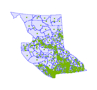
The BC Voting Area dataset is a convenient test case, since it has lots of large polygons (shown here with interior points computed).
The query is about as simple as it gets:

   select ST_PointOnSurface(geom) from ebc.voting_area;

Here's the query timings comparison, using the improved GEOS code and the previous implementation:

Data size Time Time
OLD
Improvement Time
ST_Centroid
5,658 polygons
(2,171,676 vertices)
341 ms 4,613 ms x 13 369 ms

As expected, there is a dramatic improvement in performance.  The improved ST_PointOnSurface runs 13 times faster than the old code.  And it's now as fast as ST_Centroid.  It's also more robust and tolerant of invalid input (although this test doesn't show it).

This should show up in PostGIS in the fall release (PostGIS 3 / GEOS 3.8).

On to the next improvement... (and also gotta update the docs and the tutorial!)

Thursday, 21 February 2019

Better/Faster Interior Point for Polygons - now in GEOS

As a gentle introduction to GEOS development I took on the task of porting the recent improvements to the JTS InteriorPointArea algorithm.   This is a fairly small chunk o'code, but it touches most of the aspects of GEOS development process: build chain, debugging, unit tests, and infra (source control and build farm).  It also has the advantage that the JTS code was still hot off the keyboard and (almost) unreleased, so it was a chance to see if any cross-fertilization would blossom from working on the two projects jointly.

Skipping lightly over the details of my (somewhat painful) GEOS learning curve, I'm delighted to say that the code has landed in master and is basking in the green glow from the build bot badges.

And now the whole point of the exercise: how much better is the new code in GEOS? 

It exhibits the expected improvement in robustness, since a GEOS test which actually depended on a thrown TopologyException (due to the now-removed call to Geometry::intersection() ) had to be modified to handle a successful return.

Most importantly, there is a dramatic improvement in performance.  Here's some numbers from running the GEOS InteriorPointArea performance test:

Data size Time Time
OLD
Improvement Time
Centroid
100 .8 ms 86 ms x 100 1 ms
1000 6 ms 144 ms x 24 12 ms
10,000 55 ms 672 ms x 12 107 ms
100,000 508 ms 6,714 ms x 13 961 ms
1,000,000 5,143 ms 73,737 ms x 14 11,162 ms

Some observations:
  • The performance test uses synthetic data (sine stars).  Real-world datasets are likely to show significantly better times ( 80x better in some cases, based on JTS timings)
  • The largest improvement is for small geometries, which is nice since these are more common
  • InteriorPoint is now actually faster than the Centroid computation.  This is also good news, since users were often tempted to try and use centroids instead of interior points, despite the known issues.
Future Work

Running the identical performance test in JTS is still faster, by roughly 5x.  This may be due to the advantages of JIT compilation and memory management.  It may also indicate there is room for improvement by making GEOS smarter about data handling.

Tuesday, 12 February 2019

Better and Faster Interior Point for Polygons in JTS/GEOS

A humble workhorse of geospatial processing is the ability to compute a point which is guaranteed to lie in the interior of a polygon.  In the OGC Simple Features for SQL specification (and hence in PostGIS) this is known as ST_PointOnSurface.  In JTS/GEOS it is called getInteriorPoint, for historical reasons [1].

Interior points for country boundaries

There are some important use cases for this capability:
  • Constructing a "proxy point" for a polygon to use in drill-down spatial query.  This has all kinds of applications:
  • Cartographic rendering including:
    • Creating leader lines
    • Placing labels for polygons (for which it is a quick solution but not necessarily a quality one.  More on this in a later post)
There is a variety of ways that have been proposed to compute interior points: triangulation, sampling via random or grid points, medial axis transform, etc.  These all involve trade-offs between location quality and performance [2].  JTS uses an approach which optimizes performance, by using a simple scan-line algorithm:

JTS Scan-Line Interior Point Algorithm
  1. Determine a Y-ordinate which is distinct to every polygon vertex Y-ordinate and close to the centre of the vertical extent
  2. Draw a scan line across the polygon and determine the segments of intersection
  3. Choose the interior point as the midpoint of the widest intersection segment
Locating a polygon interior point along a scan-line

The current code has been in the JTS codebase since the release of the very first version back in 2001.  It is elegantly simple, but is quite non-optimal, since it uses the overlay intersection algorithm.  This is overkill for the computation of the scan-line intersection segments.  It also has a couple of serious drawbacks: slow performance, and the requirement that the input polygon be valid.  These are not just theoretical concerns.  They have been noticed in the user community, and have caused client projects to have to resort to awkward workarounds.  It's even documented as a known limitation in PostGIS.

Thanks to Crunchy Data recognizing the importance of geospatial, we've been able to look into fixing this.  It turns out that a relatively simple change makes a big improvement.  The scan-line intersections can be computed via a linear-time scan of the polygon edges.  This works even for invalid input (except for a few pathological situations).
Interior points of invalid polygons
(LH invalid polygon shows suboptimal point placement)

Best of all, it's much faster - providing performance comparable to the (less useful) centroid computation.  The performance results speak for themselves:

Dataset # polys # points Time Prev
time
Improvement
World countries
244
366,951 25 ms 686 ms
x 27
Land Cover 64,090 366,951 78 ms 6.35 s
x 81

This has been committed to JTS.  It will be ported to GEOS soon, and from there should show up in PostGIS (and other downstream projects like QGIS, Shapely, GDAL, etc etc).

More Ideas

Some further improvements that could be investigated:
  • Use the centroid to provide the Y-ordinate.  This is probably better in some situations, and worse in others.  But perhaps there's a fast way to choose the best one?
  • Use multiple scan-lines (both vertical and horizontal)
  • Provide better handling of short/zero-width scan-line intersections
  • Support clipping the interior point to a rectangle.  This would provide better results for cartographic labelling


[1] JTS was based on the original OGC SFS specification (version 1.1).  The spec actually does include a method Surface.pointOnSurface.  The reason for the different choice of name is lost to time, but possibly the reasoning was that the JTS function is more general, since it handles all types of geometry.  (One of the design principles of JTS is Geometric Uniformity, AKA No Surprises.  Wherever possible spatial operations are generalized to apply to all geometric types. There is almost always a sensible generalization that can be defined, and it's often quite useful.)

[1a] Also, the acronym IPA is much better than the one for PointOnSurface.

[2] Apparently Oracle has decided to provide blazingly fast performance by simply returning a point on the boundary of the polygon.  Thus proving the maxim that for every problem there is an solution which is simple, fast, and dead wrong.


Saturday, 2 February 2019

Joining Crunchy Data to work on PostGIS

I'm happy to announce that I am taking a position with Crunchy Data as a Senior Geospatial Engineer.  I'm working alongside fellow Victorian geospatial maven extraordinaire Paul Ramsey, as the core of a proposed Geospatial Data Centre of Excellence.

Our mission statement is simple:  make PostGIS bigger, better, faster!

  • Bigger - more spatial algorithms and functions
  • Better - enhance existing functionality to make it easier to use, more powerful, and more robust
  • Faster - keep looking for algorithmic optimizations and ways to use the power of Postgres to make spatial processing faster

A lot of this work will involve enhancements to the core GEOS geometry library.  Part of the goal is to keep JTS and GEOS aligned, so this should produce a nice boost to JTS as well.

Having been lurking in the background for many years now, I'm stoked to be (finally) able to work directly on PostGIS.  And I'm excited to be part of the Crunchy team. They have some of the leading Postgres experts in-house, so I'm expecting that it will be a great learning experience.  And their client list promises to expose us to some fascinating large-scale use cases for spatial data processing, which can only be good for the power and robustness of PostGIS.

I'm also looking forward to re-engaging with the geospatial open source community, and learning more about the (even bigger) open source Postgres community.  Great things lie ahead!


Monday, 28 January 2019

Hilbert and Morton Curves in JTS

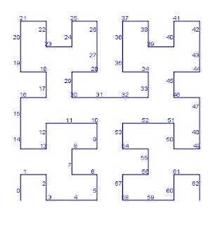
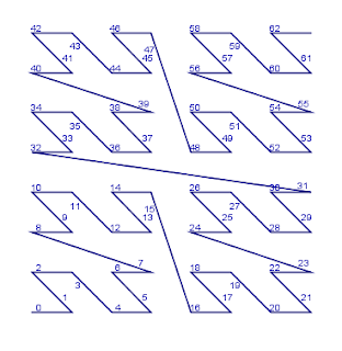
I just landed a JTS pull request for Hilbert and Morton (Z-order) codes and curves.
Hilbert Curve of level 3
Morton Curve of level 3

Apart from pretty pictures of fractals, the goal is to support experimenting with Packed Hilbert R-trees, as an alternative to the current Sort-Tile-Recursive packing strategy (implemented as STRtree in JTS).  STRtrees are heavily used to speed up spatial algorithms inside JTS (and externally as per recent report). So if Hilbert curve-based packing provides better performance that would be a big win.


Thursday, 17 January 2019

Fun wit JEQL: Hilbert Curves

Hilbert Curve of order 4:


Hilbert Curve of order 6:
Code is in the JEQL script repo.

import jeql.std.function.HashFunction;

hilbertOrder = 6;
side = Val.toInt( Math.pow(2, hilbertOrder) );
count = side * side;

radius = 1;

t = select * from Generate.sequence( 0, count-2 );

t = select i, geom: Geom.buffer(hilbertEdge, 0.4)
let 
hilbertPt1 = HashFunction.hilbertPoint(hilbertOrder, i),
hilbertPt2 = HashFunction.hilbertPoint(hilbertOrder, i+1),
hilbertEdge = Geom.createLineFromPoints( hilbertPt1, hilbertPt2 )
from t;

t1 = select *,
styleFill: clr, styleStroke: clr, styleStrokeWidth: 1
let
clr = Color.toRGBfromHSV(Val.toDouble(i) / count, 1, 1)
from t;
Mem t1;

The function hilbertPoint uses the efficient algorithm from http://threadlocalmutex.com/.  Code is on Github.