Coverage Cleaning in JTS

The JTS Topology Suite has been rolling out the capability to manage polygonal coverages.  It supports modelling polygonal coverages as arrays of discrete polygonal geometries.  This is simple to work with and allows using all of the wide variety of JTS algorithms.  Coverage topology allows operations such as CoverageSimplifier and CoverageUnion to be highly performant and effective.

The key requirement for coverage operations is that the input is a valid polygonal coverage.  JTS provides the CoverageValidator to check a dataset to see if it is a valid coverage, and provide full information on the location of topology errors.  However, this leaves the question of how to convert a dataset with errors into a valid coverage.  

There are two options for fixing coverages: manual editing, and automated cleaning.  CoverageValidator provides information to identify the location of all errors. However, manually fixing them is time-consuming, and difficult in environments which lack convenient editing tools. And of course it simply isn't feasible in automated workflows.

What users really want is automated coverage cleaning.  This is a major pain point (witness the numerous questions about how to do this; for example, this and this and this).  Clearly, cleaning coverages is considered critical!

There are several existing tools to do this:

• mapshaper is perhaps the most popular tool currently.  It supports snapping to improve dataset quality, along with overlap and gap merging.  It is written in Javascript, which provides surprisingly good performance, but makes it awkward to integrate in other tools.
• pprepair is an academically-advanced algorithm which uses triangulation as the basis for cleaning.  It relies on CGAL, which limits appeal for integration
• GRASS v.clean is a long-standing cleaning tool with an extensive set of options for carrying out various kinds of cleaning

But in the JTS/GEOS ecosystem it's been a gap that needs filling (so to speak).  So I'm excited to announce the the arrival of the JTS CoverageCleaner.

JTS CoverageCleaner class

The JTS CoverageCleaner class provides the essential capabilities of cleaning polygonal data to form a valid coverage:

• Snapping: snapping vertices and lines eliminates small discrepancies and narrow gaps, and improves the robustness of subsequent processing
• Overlap Merging: of two or more polygons are merged with a neighbouring polygon.  The merge target can be chosen to be the neighbour with the longest shared border, the largest or smallest area, or the one with minimum input index (which allows priority-based merging).
• Gap Detection and Merging: Gaps are defined as enclosed empty areas with width less than a distance tolerance.  Width is computed as the diameter of the Maximum Inscribed Circle of the gap polygon. (This is an improvement over other tools, which only offer cruder area or roundness-metric tests to identify gaps to be merged.) Gaps can be filled and merged with an adjacent polygon. 

The output of the cleaner is a valid polygonal coverage that contains no overlaps and no gaps narrower than the given tolerance.  The merged overlaps and gaps are also available for visualization and QA purposes.

Other aspects of cleaning data are provided by separate JTS classes.  Invalid polygonal geometries can be preprocessed with GeometryFixer to repair them.  CoverageSimplifier can be used to reduce the vertex size of cleaned datasets.  And a forthcoming coverage precision reducer will allow controlling the amount of precision maintained (which can reduce the space required for some storage formats).

Algorithm Description

This is a good example of how the breadth of JTS capabilities makes it easier to develop new algorithms:

• the SnappingNoder was developed for OverlayNG, and turned out to be ideal for eliminating minor errors and providing a robust basis for the rest of the process
• the Polygonizer allows fast recreation of a coverage topology from the noded linework
• Spatial indexes (STRtree and Quadtree) and the fast predicates of RelateNG provide performance for operating in the discrete geometric domain
• the new fast MaximumInscribedCircle.isRadiusWithin predicate allows using polygon width for gap detection

The cleaning algorithm works as follows:

Input

The input is an array of valid polygonal geometries.  This is the same structure used in other coverage operations.  However, it may or may not not have valid coverage topology.  The array position acts as an implicit identifier for the coverage elements.

Snapping and Noding

Input linework is extracted and noded using the SnappingNoder.  Snapping vertices and lines using a distance tolerance eliminates small discrepancies and narrow gaps, and improves the robustness of noding.  By default a very small snapping distance is used (based on the diameter of the dataset.)  The user can specifiy a custom snapping distance. Larger distances can be more effective at cleaning the linework.  However, too large a distance can introduce unwanted alteration to the data.

Polygonizing and Resultant Categorization

The noded linework is polygonized using the Polygonizer. This forms a clean topology of resultant polygons.  Resultant polygons are associated with their parent input polygon(s) via their interior points and point-in-polygon tests. Resultants are categorized according to their number of parents:

• Result area:  one parent (which identifies the associated input polygon)
• Overlap: multiple parents
• Gap: no parents

Overlap Merging

Overlaps are always merged, since they violate coverage topology.  They are merged with an adjacent result area chosen via a specified merge strategy.  The strategy indicates whether the merge target is chosen to be the neighbour with the longest shared border, the largest or smallest area, or the one with minimum input index (which allows priority-based merging).

Gap Detection and Merging

Gaps in the created coverage do not invalidate coverage topology, but they are often an artifact of invalidities, or may be errors in the original linework.  For this reason a distance tolerance can be used to select gaps to be merged.  Gaps which are narrower than the width tolerance are merged with the neighbour result area with longest shared border.  The width of the gap polygon is determined by the diameter of the MaximumInscribedCircle.  (This is an improvement over other tools, which only provide cruder area or roundness-metric tests to identify gaps.)

Identifying narrow gaps to be merged via Maximum Inscribed Circle radius

Output

The output is an array of the same size as the input array.  Each element is the cleaned version of the corresponding input element, and the entire array forms a valid polygonal coverage.  Due to snapping very small inputs may disappear.  The output may still contain gaps larger than the gap width tolerance used.  (One way to to detect these is to union the coverage - the result will have holes where gaps exist.) Cleaning can be re-run with a larger tolerance to remove more gaps.

Examples

Given the number of tools available to clean polygonal coverages, it's slightly surprising that you don't have to look hard to find datasets containing coverage topology errors.  But that's good for testing!  Here are some examples demonstrating the behaviour and performance of CoverageCleaner.

Example 1: Montana County Commissioner Districts

This is one of the jurisdiction coverages available here.  The dataset contains 177 areas with 470,229 vertices.  Running CoverageValidator finds errors at over 12,000 locations:

Zooming in on an area containing errors using the JTS TestBuilder Magnify Topology tool shows that errors are caused by small misalignments in the linework of adjacent polygons, creating both gaps and overlaps:

Running the Coverage Cleaner with the default snapping tolerance and a gap width of 10 produces a clean coverage in 0.88 seconds.  The effect of snapping removes 2043 overlaps and 1793 gaps.  After topology building, merging removes a further 14 overlaps and 12 gaps. (This is determined by running the cleaning process with both default snapping tolerance and a tolerance of 0, and counting the merged overlaps and gap polygons available from the cleaner instance.)

Example 2: Communes in France Department 71

This example is a dataset representing communes in the French department 71 (Saône-et-Loire).  It may have been assembled by aggregating cadastral parcels, which is a common cause of discrepancies due to different data origins.  The dataset contains 564 areas with 612,238 vertices.  Validating the coverage reveals over 362,000 error locations (and in fact this doesn't represent all of the gaps present).

Zooming shows some example overlaps and gaps. Magnify Topology is not needed since the discrepancies are on the order of metres in size.

Running the Coverage Cleaner with default snapping tolerance and a Gap Width of 50 produces a clean coverage in 23 seconds.  The slower performance over Example 1 is due to the much larger number of gaps and overlaps: 29,307 overlaps and 28,409 gaps.  They are almost all too wide to be handled by snapping, so they must be merged, which requires more processing.

Here's a before-and-after view of an area of the cleaned coverage, showing the effect of merging gaps and overlaps:

Gap Merging Quality Issues

Given the size and number of issues in the France-71-communes dataset, it's not surprising that it exhibits two known problems with the current gap merging strategy: spikes creating by merged gaps, and unmerged narrow gap parts.

Here is an example of how merging a gap to an adjacent polygon can create a spike in the result polygon.  (Merging overlaps does not produce these kinds of errors, since the overlap was part of the merge target originally.)

This is an example of a wide gap which is not merged, but which has narrow portions which could be "clipped off" and merged:

Improving the quality of gap merging is an area for further research and development.

GEOS and PostGIS Ports

As usual, this work will be ported to GEOS soon, and then exposed in PostGIS as a new coverage function,  It should also show up in downstream projects such as Shapely and hopefully QGIS.

Further Enhancements

Overlap and Gap Handling

There are other possibilities for controlling overlap merging and gap filling.  Choosing merge targets could be determined by a priority value on each input area.  Gaps could be determined by area or roundness measure criteria, as provided in other systems (although they seem less precise than using polygon width.)     

Gap Partitioning and Spike Removal 

Gaps which are very long can extend along multiple polygons. If a gap of this nature is merged to single polygon it will create a spike in the merged polygon.  Instead, it would be better to partition the gap into multiple pieces at polygon nodes and merge the parts separately.

A more complex situation is when a gap contains both narrow and wide portions.  An example of this is a parcel coverage with blocks separated by narrow streets and wider intersections and squares.  Ideally the narrow parts could be partitioned off and merged, leaving the wide portions unmerged.  

Gore Removal

Gores are narrow "inlets" along the border of in a coverage.   They have a similar shape to gaps, but since they are not closed they are not identified as gaps by the cleaning process.  They could be identified by a different process, closed off, and then merged (ideally with partitioning as discussed above).

Coverage precision reduction

A common requirement in data management is to reduce the precision of data coordinates.  For coverages this cannot be done piecewise, but must be performed as a global operation over the entire coverage, since rounding coordinates independently can create line intersections.  The SnapRoundingNoder provides an effective way of doing this.

Validating Polygonal Coverages in JTS

The previous post discussed polygonal coverages and outlined the plan to support them in the JTS Topology Suite.  This post presents the first step of the plan: algorithms to validate polygonal coverages.  This capability is essential, since coverage algorithms rely on valid input to provide correct results.  And as will be seen below, coverage validity is usually not obvious, and cannot be taken for granted.  

As described previously, a polygonal coverage is a set of polygons which fulfils a specific set of geometric conditions.  Specifically, a set of polygons is coverage-valid if and only if it satisfies the following conditions:

• Non-Overlapping - polygon interiors do not intersect
• Edge-Matched (also called Vector-Clean and Fully-Noded) - the shared boundaries of adjacent polygons has the same set of vertices in both polygons

The Non-Overlapping condition ensures that no point is covered by more than one polygon.  The Edge-Matched condition ensures that coverage topology is stable under transformations such as reprojection, simplification and precision reduction (since even if vertices are coincident with a line segment in the original dataset, this is very unlikely to be the case when the data is transformed).  

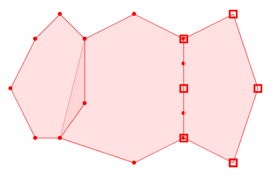
An invalid coverage which violates both (L) Non-Overlapping and (R) Edge-Matched conditions (note the different vertices in the shared boundary of the right-hand pair)

Note that these rules allow a polygonal coverage to cover disjoint areas.  They also allow internal gaps to occur between polygons.  Gaps may be intentional holes, or unwanted narrow gaps caused by mismatched boundaries of otherwise adjacent polygons.  The difference is purely one of size.  In the same way, unwanted narrow "gores" may occur in valid coverages.  Detecting undesirable gaps and gores will be discussed further in a subsequent post. 

Computing Coverage Validation

Coverage validity is a global property of a set of polygons, but it can be evaluated in a local and piecewise fashion.  To confirm a coverage is valid, it is sufficient to check every polygon against each adjacent (intersecting) polygon to determine if any of the following invalid situations occur:

• Interiors Overlap:
• the polygon linework crosses the boundary of the adjacent polygon
• a polygon vertex lies within the adjacent polygon
• the polygon is a duplicate of the adjacent polygon
• Edges do not Match:
• two segments in the boundaries of the polygons intersect and are collinear, but are not equal 

If neither of these situations are present, then the target polygon is coverage-valid with respect to the adjacent polygon.  If all polygons are coverage-valid against every adjacent polygon then the coverage as a whole is valid.

For a given polygon it is more efficient to check all adjacent polygons together, since this allows faster checking of valid polygon boundary segments.  When validation is used on datasets which are already clean, or mostly so, this improves the overall performance of the algorithm.  

Evaluating coverage validity in a piecewise way allows the validation process to be parallelized easily, and executed incrementally if required.

JTS Coverage Validation

Validation of a single coverage polygon is provided by the JTS CoveragePolygonValidator class.  If a polygon is coverage-invalid due to one or more of the above situations, the class computes the portion(s) of the polygon boundary which cause the failure(s).  This allows the locations and number of invalidities to be determined and visualized.

The class CoverageValidator computes coverage-validity for an entire set of polygons.  It reports the invalid locations for all polygons which are not coverage-valid (if any). 

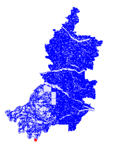
Using spatial indexing makes checking coverage validity quite performant.  For example, a coverage containing 91,384 polygons with 10,474,336 vertices took only 6.4 seconds to validate.  In this case the coverage is nearly valid, since only one invalid polygon was found. The invalid boundary linework returned by CoverageValidator allows easily visualizing the location of the issue.

A polygonal dataset of 91,384 polygons, containing a single coverage-invalid polygon

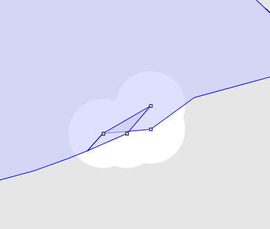
The invalid polygon is a tiny sliver, with a single vertex lying a very small distance inside an adjacent polygon.  The discrepancy is only visible using the JTS TestBuilder Reveal Topology mode.

The size of the discrepancy is very small.  The vertex causing the overlap is only 0.0000000001 units away from being valid:

[921]  POLYGON(632)

[922:4]  POLYGON(5)

Ring-CW  Vert[921:0 514]  POINT ( 960703.3910000008 884733.1892000008 )

Ring-CW  Vert[922:4:0 3]  POINT ( 960703.3910000008 884733.1893000007 )

This illustrates the importance of having fast, robust automated validity checking for polygonal coverages, and providing information about the exact location of errors.

Real-world testing

With coverage validation now available in JTS, it's interesting to apply it to publicly available datasets which (should) have coverage topology.  It is surprising how many contain validity errors.  Here are a few examples:

Source	City of Vancouver
Dataset	Zoning Districts

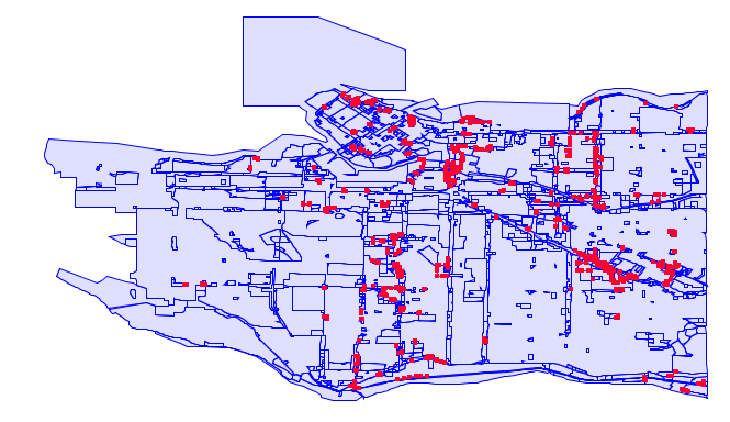
This dataset contains 1,498 polygons with 57,632 vertices. There are 379 errors identified, which mainly consist of very small discrepancies between vertices of adjacent polygons.

Example of a discrepant vertex in a polygon

Source	British Ordnance Survey OpenData
Dataset	Boundary-Line
File	unitary_electoral_division_region.shp

This dataset contains 1,178 polygons with 2,174,787 vertices. There are 51 errors identified, which mainly consist of slight discrepancies between vertices of adjacent polygons. (Note that this does not include gaps, which are not detected by CoverageValidator.  There are about 100 gaps in the dataset as well.)

An example of overlapping polygons in the Electoral Division dataset

Source	Hamburg Open Data Platform
Dataset	VerwaltungsEinheit (Administrative Units)

The dataset (slightly reduced) contains 7 polygons with 18,254 vertices.  Coverage validation produces 64 error locations.  The errors are generally small vertex discrepancies producing overlaps.  Gaps exist as well, but are not detected by the default CoverageValidator usage.

An example of overlapping polygons (and a gap) in the VerwaltungsEinheit dataset

As always, this code will be ported to GEOS.  A further goal is to provide this capability in PostGIS, since there are likely many datasets which could benefit from this checking.  The piecewise implementation of the algorithm should mesh well with the nature of SQL query execution.

And of course the next logical step is to provide the ability to fix errors detected by coverage validation.   This is a research project for the near term.

UPDATE: my colleague Paul Ramsey pointed out that he has already ported this code to GEOS.  Now for some performance testing!

Polygonal Coverages and Operations in JTS

An important concept in spatial data modelling is that of a coverage.  A coverage models a two-dimensional region in which every point has a value out of a range (which may be defined over one or a set of attributes).  Coverages can be represented in both of the main physical spatial data models: raster and vector.  In the raster data model a coverage is represented by a grid of cells with varying values.  In the vector data model a coverage is a set of non-overlapping polygons (which usually, but not always, cover a contiguous area).  

This post is about the vector data coverage model, which is termed (naturally) a polygonal coverage. These are used to model regions which are occupied by discrete sub-regions with varying sets of attribute values.  The sub-regions are modelled by simple polygons.  The coverage may contain gaps between polygons, and may cover multiple disjoint areas.  The essential characteristics are:

• polygon interiors do not overlap
• the common boundary of adjacent polygons has the same set of vertices in both polygons.

There are many types of data which are naturally modelled by polygonal coverages.  Classic examples include:

• Man-made boundaries
• parcel fabrics
• political jurisdictions
• Natural boundaries
• vegetation cover
• land use

A polygonal coverage of regions of France

Topological and Discrete Polygonal Coverages

There are two ways to represent polygonal coverages: as a topological data structure, or as a set of discrete polygons.  

A coverage topology consists of linked faces, edges and nodes. The edges between two nodes form the shared boundary between two faces.  The coverage polygons can be reconstituted from the edges delimiting each face.  

The discrete polygon representation is simpler, and aligns better with the OGC Simple Features model.  It is simply a collection of polygons which satisfy the coverage validity criteria given above.

Most common spatial data formats support only a discrete polygon model, and many coverage datasets are provided in this form.  However, the lack of inherent topology means that datasets must be carefully constructed to ensure they have valid coverage topology.  In fact, many available datasets contain coverage invalidities.  A current focus of JTS development is to provide algorithms to detect this situation and provide the locations where the polygons fail to form a valid coverage.

Polygonal Coverage Operations

Operations which can be performed on polygonal coverages include:

• Validation - check that a set of discrete polygons forms a valid coverage
• Gap Detection - check if a polygonal coverage contains narrow gaps (using a given distance tolerance)
• Cleaning - fix errors such as gaps, overlaps and slivers in a polygonal dataset to ensure that it forms a clean, valid coverage
• Simplification - simplify (generalize) polygon boundary linework, ensuring coverage topology is preserved
• Precision Reduction - reduce precision of polygon coordinates, ensuring coverage topology is preserved
• Union - merge all or portions of the coverage polygons into a single polygon (or multipolygon, if the input contains disjoint regions)
• Overlay - compute the intersection of two coverages, producing a coverage of resultant polygons 

Implementing polygonal coverage operations is a current focus for development in the JTS Topology Suite.  Since most operations require a valid coverage as input, the first goal is to provide Coverage Validation.  Cleaning and Simplification are priority targets as well.  Coverage Union is already available, as is Overlay (in a slightly sub-optimal way).  In addition,  a Topology data structure will be provided to support the edge-node representation.  (Yes, the Topology Suite will provide topology at last!).  Stay tuned for further blog posts as functionality is rolled out.

As usual, the coverage algorithms developed in JTS will be ported to GEOS, and will thus be available to downstream projects like PostGIS.