Thursday, 14 July 2011

Would you be lost without it?

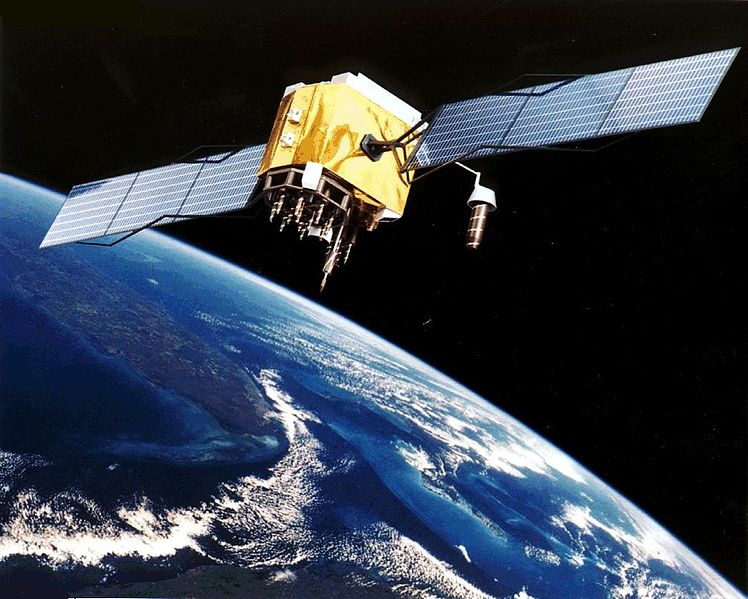
Nowadays GPS is ubiquitous in electronic gadgets (no electric toothbrush is complete without it!) GPS is a classic example of iceberg technology 1. An output which in one sense verges on trivial - two numbers! - in fact relies on a huge unseen infrastructure of technology, physics, organizations, and yes, government funding.

The UK Telegraph has an interesting article on GPS 2 covering some of the technical, scientific, historic and political background to the system.


On a side note, I'm happy to observe that statements like this aren't as common as they used to be:

Slightly worryingly, when I was invited to watch a “contact” in another control room earlier in the day, the software crashed and a familiar, blue Microsoft Windows screen appeared on the wall


Notes:
  1. yes I made this up. My entry for Internet memedom!
  2. don't worry, it's still safe to use your cellphone after visiting this site

Sunday, 26 June 2011

JTS 1.12 released

JTS 1.12 has been released, and is now available for download at SourceForge.

Some highlights of this release include:
... along with many other features, enhancements and fixes.


Single-Sided Buffer

Wednesday, 8 June 2011

Apple walls getting higher

ZDNet has an interesting long view on the Apple iCloud announcement. Money quote:
The mobile world is moving away from the chock-full-o’-content web and increasingly becoming a world of closed pipes of content, with Apple, Google, HP and Microsoft regulating the flow. Tech fiefdoms scattered across a vast open land have expanded into warring nation-states with adjacent borders. The Mac vs. PC vs. Linux argument from the early days of consumer computing has lost a great deal of its luster in recent years with the development of cloud computing on the open web, but the concept of platform wars is quickly making up for lost ground with the development of cloud computing in the closed mobile space.
I've always found the Apple walled garden a bit scary in its restrictions. Now the walls are getting higher and thicker - and other vendors will be following suit as fast as they dare.

I don't find Google's garden as threatening, for some reason. Perhaps because they have a different business model, based on page views rather than selling devices or software. For now that encourages them to not put any limits on where and how you access their services. But will that change if the Chromebook takes off? Is the fact that Honeycomb is not open source a tiny black cloud on the horizon?


Monday, 6 June 2011

Java gets Reheated at OSCON

It's good to see that O'Reilly is adding a Java flavour to the OSCON conference. They have a good blog post highlighting why they think Java (and the JVM) is still one of the most important programming platforms around, especially for open source development.


Some of the interesting Java projects that will be covered at the conference are:
  • Incanter, a Clojure-based statistics library (this project is particularly interesting to me, since it overlaps with some of the target space of JEQL)
  • Gradle, a Groovy DSL for building, testing, and deploying software
  • Jenkins, a continuous integration platform
  • Neo4J, a graph database
Some may think that Java is entering the Red Giant phase of language evolution, but it still has the capacity to throw off some powerful solar flares. The longer the coffee pot sits on the stove, the stronger it gets...

Thursday, 19 May 2011

JTS arrives in JavaScript

As I predicted back in 2008, JTS has now colonized the JavaScript ecosystem, thanks to the work of Bjorn Hartell on JSTS. At least, the project has been launched - it's a bit unclear as to how much functionality is actually there.

I hope to see some slick browser-based UI clients pop up, using Canvas or perhaps SVG?

The language scorecard for JTS now looks like:

[Update: Jan 31 2013] - Added R to the list

Wednesday, 4 May 2011

FOSS4G is the place to be!

FOSS4G 2011 is happening in Denver this September.


I've submitted two abstracts for presentations:


Spatial Processing using JEQL

JEQL is a simple yet powerful language designed for expressing spatial (and non-spatial) processes. It follows the Table-Oriented Programming paradigm and provides a SQL-like query language. This talk gives an overview of JEQL and show some examples of its use.


What's New in JTS

The JTS Topology Suite has had numerous improvements in the past few versions. These include performance improvements, bug fixes and new functionality such as Delaunay Triangulation, Single-Sided Buffers, and Hausdorff Distance. This talk will discuss the new features, and demonstrate them using the JTS TestBuilder utility. Potential further features will be presented for discussion.


Vote early, vote often - and vote for me!

See you in Denver....


Friday, 8 April 2011

Polygon Triangulation via Ear-Clipping with Delaunay Refinement

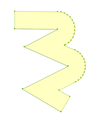
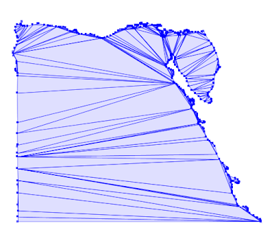
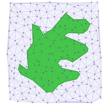
After this thread on the JTS list Michael Bedward was inspired to create a polygon triangulation algorithm using the Ear-Clipping approach. Standard Ear-Clipping algorithms don't handle polygons with holes, but Michael made a nice extension to do this. (David Eberly has a good write-up on this subject here, and of course there's always Wikipedia). One problem with ear-clipping is that it produces sub-optimal triangulations (in the the sense that it creates lots of very skinny triangles, which are visually and computationally unappealing). I suggested that he add a refinement step based on "flipping triangles" to improve the quality of the output triangle mesh. This is similar to the approach used in Delaunay triangulation algorithms, and in fact it turns out that a good flipping criteria is to test for the Delaunay condition. (Two adjacent triangles which form a convex quadrilateral are Delaunay if neither lies in the circumcircle of the other. Wikipedia has a nice visual explanation). This code will get added to JTS in the next release. In the meantime, here's some cool pictures showing how it works. A gnarly test polygon:
Before refinement
After refinement
A country that has been in the news recently:
Before refinement
After refinement
Update (Nov 1, 2021): JTS now has Polygon Triangulation code.  See this post for details.

Dynamic Views in Google Blogs

Check out the cool new Dynamic Views feature for Google Blogs. I'm not sure how useful this is actually going to be for readers (especially since you have to do URL editing to invoke them - WTB!? (Where's The Button 8^)

But they sure look purty. Here's a shot of the Flipcard view:

Thursday, 7 April 2011

Slope/Aspect/Elevation using JTS

David Skea is a longtime colleague, JTS contributor, and all-around geospatial guru. He's developing a Slope/Aspect/Elevation service to be used in forestry-related applications here in British Columbia. His work is a nice example of using JTS to perform real-world spatial processing.

The key to computing slope, aspect and elevation is to have a Digital Elevation Model (DEM) available for the terrain in the area of interest. In this case, the terrain data is provided by the TRIM irregular DEM, which is a dataset of over 500 million mass points covering all of British Columbia. To compute the required values for a given polygon, the first step is to extract only the mass points in the immediate region of the polygon (i.e. using the polygon envelope with a suitable buffer distance. The JTS Delaunay Triangulation API is used to compute a TIN triangulation from the TRIM mass points.


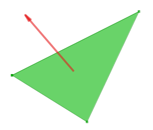
Using a JTS PointOnGeometryLocator, the triangles whose centroids lie in the polygon are selected. Since each mass point has an elevation value, each TIN triangle is located in 3D space. The normal vector can be computed for each triangle, which provides the slope and aspect values. The elevation is the height of the triangle centroid.

The SEA values for the triangles are averaged to compute the overall slope, aspect and elevation value for the polygon.

Here's a screenshot showing the results, using Google Earth as a convenient 3D visualization tool (click for full-size image).

Thursday, 3 March 2011

GeoGeeks presentation on Geometry Libraries

Paul Ramsey has been doing his usual excellent work of promoting geo-geekery by setting up a Victoria GeoGeeks Meetup. Tonight I gave a presentation on Geometry Libraries for Fun and Profit.


I was intending to give it back-to-back with a presentation on JTS, to make the whole subject more concrete - but I rambled on for so long I was yanked from the stage before I could start on the second one! That's actually good, since it will give me time to polish up the presentation a bit more. In the meantime, the current slide deck is here: JTS - A Libary for Geometry Processing.

Tuesday, 11 January 2011

Charting with JEQL

SQL has an elegant syntax for grouping and aggregating data. Java has powerful libraries for charting and graphing (like JFreeChart). JEQL has easy handling of tabular data. These go together like chocolate and peanut butter - and, um, more chocolate. Put them all together and you get this code:

CSVReader troute hasColNames: file: "routeLine2.csv";

tCityCount = select count(*) cnt, fromCity city
from troute
group by fromCity
order by cnt desc;

tdata = select city key, cnt value from tCityCount limit 20;

Chart type: "bar"
data: tdata
extrude:
color: "00c0f0"
showItemLabels:
xAxisTitle: "Top Cities by Originating Air Routes"
xAxisLabelRotation: -0.5
width: 1000
file: "cityRoutes.png";


producing this graph:


This uses the same air routes dataset created in a previous example, with a simple grouped summary to show the 20 cities with the most air routes originating in them.

JFreeChart is a bit notorious for being hard to use, but the JEQL command hides all the gory details behind a much simpler (but still powerful) Chart command interface. Currently Bar, XY, and Pie charts are supported. It will be easy to add other chart types as required.

Also on the ToDo list is to provide an option to emit Google Chart URLs, using the same set of options (at least, the ones that are applicable - and maybe some new ones).

Note: this is an experimental extension, which is not in a final state in the current JEQL release.

Thursday, 6 January 2011

JEQL 0.9 released

Good news for those who wanted to try out the geodetic air routes JEQL script. The script requires JEQL version 0.9 to run. This version is now available for download.

Tuesday, 28 December 2010

Goodbye LAMP, hello SMAQ

A great article on the emerging SMAQ stack for big data.

I wonder if PIG does spatial?

Monday, 27 December 2010

Diving deep into Computational Geometry

For a deep dive into the bracing waters of cutting-edge computational geometry, check out the online proceedings of the Canadian Conference of Computational Geometry.


Do NOT expect to see these algorithms appear in JTS anytime soon!

Sunday, 26 December 2010

Visualizing geodetic information with JEQL

The geo-blogosphere has been buzzing about the global Facebook friends visualization. This was done by Paul Butler using an R script and some clever techniques for working with geodetic data.


This kind of lightweight spatial analysis and visualization is squarely in the target zone for JEQL, so I thought I'd try something similar.

Of course I don't have access to the Facebook friends dataset, so I needed some other suitable dataset of global-scale links. An obvious candidate is airline routes. Luckily there is an excellent open data repository called OpenFlights. It has datasets which are tables of airport locations and air routes between airports:

airports.dat:

1,"Goroka","Goroka","Papua New Guinea","GKA","AYGA",-6.081689,145.391881,5282,10,"U"
2,"Madang","Madang","Papua New Guinea","MAG","AYMD",-5.207083,145.7887,20,10,"U"
3,"Mount Hagen","Mount Hagen","Papua New Guinea","HGU","AYMH",-5.826789,144.295861,5388,10,"U"
...

routes.dat:

0B,1542,AGP,1230,BBU,1650,,0,738
0B,1542,ARW,1647,BBU,1650,,0,340
0B,1542,BBU,1650,AGP,1230,,0,738
...

The first step is to prepare a suitable dataset for rendering. To get a table of FROM/TO locations, the routes table needs to be joined to the airport table. This is trivial to do in JEQL. After a bit of cleanup (such as removing missing data and duplicate routes), the final result is a dataset of links between airport locations using Lat/Long coordinates:

28,"Bagotville","Canada",48.330555,-70.996391,146,"Montreal","Canada",45.470556,-73.740833
29,"Baker Lake","Canada",64.298889,-96.077778,132,"Rankin Inlet","Canada",62.81139,-92.115833
30,"Campbell River","Canada",49.950832,-125.270833,119,"Comox","Canada",49.710833,-124.886667
30,"Campbell River","Canada",49.950832,-125.270833,156,"Vancouver","Canada",49.193889,-123.184444
...

As Paul found, a few other steps are needed to produce a visually appealing map:
  • Densify the route links to produce approximations to great-circle arcs
  • Break the arcs at the International Date Line to allow them to render correctly
  • Colour-theme the routes from longest to shortest using lighter colours for shorter routes
  • Render the lines with longer ones further back in the Z-order
For good measure I also added a background rendering of world land areas, as well as a country boundary layer on top. To avoid swamping the map, only routes with more than one flight listed are displayed.

The rendering is done using the following JEQL script:

CSVReader troute hasColNames: file: "routeLine2.csv";

trte = select fromCity, toCity,
Val.toDouble(fromLon) fromLon, Val.toDouble(fromLat) fromLat,
Val.toDouble(toLon) toLon, Val.toDouble(toLat) toLat
from troute;

tlines = select fromCity, toCity, line, len
with {
line = Geodetic.split180(Geodetic.arc(fromLon, fromLat, toLon, toLat, 2));
len = Geom.length(line);
}
from trte order by len desc;

tplot = select line,
Color.interpolate("f0fff0", "00c077", "004020", len / 200.0 ) lineColor,
0.4 lineWidth
from tlines;

//----- Plot world landmasses for context
ShapefileReader tworld file: "world.shp";
tworldLine = select GEOMETRY, "22222277" lineColor from tworld;
tworldFill = select GEOMETRY, "333333" fillColor from tworld;

width = 2000;
Plot width: width height: width / 2
extent: LINESTRING(-180 -90, 180 90)

data: tworldFill
data: tplot
data: tworldLine

file: "routes.png";


That's about 40 lines of code, with only 9 statements. Not a bad LOC score... Of course the heavy lifting of handling geodetic data is done by Java functions, but that's part of the point. JEQL makes it easy to link to Java code, since that's a more appropriate technology for creating performant, resusable code.

Here's the final output:
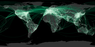


The continent outlines aren't revealed as crisply as the Facebook friends map. That's because friend links tend to be more spatially coherent than airline routes (unless your acquaintances all have private jets). But it certainly shows where the world hotspots are for air traffic. Boy, those Europeans love to fly!

Next up: the KML version...
Monday, 15 November 2010

Single-Sided Buffers in JTS

Due to popular demand I have added the capability to generate Single-Sided Buffers to JTS.

A single-sided buffer is the polygon formed by connecting a LineString to an offset curve generated on one side of the line.

Input Line

Single-Sided Buffer (width = 30)

Naturally either side can be specified, by choosing an appropriate sign for the offset distance (positive for the right side, negative for the left).

Single-Sided Buffer (width = -30)

At the moment there's a bit of a limitation, in that input linework with very narrow concave angles (relative to the buffer distance) create undesirable artifacts in the generated polygon. I'm hoping that some further thinking will come up with a way to avoid this, at least in most normal cases.

This functionality is accessed by setting an appropriate flag in the BufferParameters structure:
 BufferParameters bufParams = new BufferParameters();
bufParams.setSingleSided(true);
return BufferOp.bufferOp(geom, distance, bufParams);

Currently this code is in SVN. It will be released in JTS 1.12 (which will hopefully be shipping before year-end in Q2 2011).

Thursday, 19 August 2010

Magnifying Topology using JTS

An issue that comes up all the time in the JTS world is how to visualize the topology of geometries which have very close vertices and segments. For example, a question was recently posted on the PostGIS list about why in the situation shown below the spatial relationship predicate BLUE.contains(RED) evaluates to FALSE


At first glance it looks like the red polygon follows the boundary of the blue one exactly, which would result in BLUE.contains(RED) = TRUE. The immediate suspicion is that one of the apparently collinear points is actually in the exterior of the blue polygon. But which one? And how can this be confirmed visually?

Now it so happens that the rightmost vertex of the red polygon, which appears to be on the boundary of the blue polygon, is in fact in the its exterior - thus explaing why contains = FALSE. But it's so close to the boundary segment that no matter how far you zoom in, you can't see that this is the case. And it's certainly not obvious where to go looking for this error in the first place.

Back in the Dark Ages

The usual way to inspect these kinds of cases is is to tediously zoom in on each vertex. But this loses the visual context of the situation. And in very close cases it simply doesn't work, because the zoom factor is so great that the Swing graphics API is unable to display the scene correctly.

Zoomed in...


Zoomed further in...


Zoomed way in - FAIL!

Another alternative is a painstaking manual inspection of the coordinates of each vertex and segment (which by the way is straightforward in the TestBuilder and OpenJUMP, but can be difficult in other tools). But it's hard to convert the coordinate numbers into a mental image of the situation. And it's essentially impossible to do mentally if a vertex is near a non-rectilinear (slanted) line - in this case it's necessary to evaluate a complex mathematical algorithm to to determine the relative orientation of the vertex and line.

Into the 21st Century!

This limitation has bugged me for a long time, ever since JTS and the JCS Conflation Suite were being developed. And it keeps coming up as a question, since this kind of situation occurs a lot when overlaying polygons. Cutting new vertices into line segments almost always causes them to be non-coincident with the original segment, but with very, very small discrepancies.

So a while back I started to think about a tool that would somehow make subtle topological situations visible at convenient zoom levels. The idea has been gathering dust on the lab bench for years, but I've finally had a chance to implement it. It's now a feature in the JTS TestBuilder called Magnify Topology. Enabling it on changes the geometry view to provide easy and effective visualization of small topological differences.


Key aspects of Magnify Topology behaviour are:
  • Vertex displacement is done in a way that preserves the original topology (e.g. if a vertex is on the right side of a line it will stay on the right)
  • Vertices which are truly coincident or collinear remain unchanged in the magnified view.
  • It's easy and quick to toggle Magnify Topology on and off to compare the actual and magnified views.
Using Magnify Topology, the above case looks like this:


Now it's obvious where the red polygon violates the contains relationship! In addition, you can see that there are some very close vertices in the red polygon, that some of them are truly collinear with the blue boundary, and that the lower right red vertex is actually in the interior of the blue polygon.

Here's some more examples, showing actual and magnified views:

Example 1


Example 2

Note the truly coincident vertex along the boundary, which remains unchanged in the magnified view.


Example 3


Magnify Topology can also be used to detect and visualized differences between similar geometries (sort of like a visual geometric diff) Here's a contrived example, showing two copies of a JTS logo, in which one copy has two tiny discrepancies (in the 15th decimal place!):


Here's a more realistic real-world example:


This feature will be released in the next version of JTS. In the meantime it's available in the JTS SVN.

Monday, 2 August 2010

Cloudy Blogs

In order to try and keep abreast of the most far-reaching change to IT and computing since the invention of the PC (or the Internet, or time-sharing, or LSI, or solid-state, or commercial computing, or binary logic...), I have inaugurated a Blog Roll for sites which focus on cloud computing (in all its myriad and ever-changing forms...)

See Cloudy Blog Roll in the RH side bar --->

Friday, 9 July 2010

Is JSON the CSV of the 21st Century?

It strikes me that JSON might be the CSV of the 21st century. Consider these similarities:
  • They both use POT (plain old text) as their encoding
  • The basic datatypes are strings and numbers. JSON adds booleans and nulls - Yay for progress!
  • The only schema metadata supported is field names
JSON has the major advance of supporting hierarchical and array structures. Of course, this makes it correspondingly more difficult to parse.

CSV has stood the test of time extraordinarily well. According to good 'ol Wikipedia it's been around since at least 1967 - that's over 40 years!


And CSV is still well supported whereever tabular data is used. Let's see if JSON is still around in 2035... I suspect not, because the half-life of technologies is a lot shorter these days. (Maybe CSV is the stromatolite of file formats!)


It would be nice if JSON had a standard schema notation. (There is JSON-Schema. It copies the XML Schema idea of encoding the schema in JSON. It remains to be seen whether this makes it as easy to use and popular as XML Schema has been. 8^)

And why, o why, do field names have to be in quotes? Ok, I know why technically - they're just strings, and JSON strings need to be in quotes, because they need to be embeddable in JavaScript code. But this is a classic case of a vestigial artifact which has a detrimental effect in a new environment. Nobody should be evaling JSON as just another chunk of Javascript anyway, for obvious security reasons. And in the wider world of JSON use cases following Javascript synax is completely irrelevant.

YAML seems to have a lot advantages over JSON as a rich textual format. For instance, it has minimal use of quotes, and a richer, extensible set of datatypes including timestamps and binary (WKB, anyone?). But it's going to be pretty hard to dislodge JSON, which is solidly entrenched for all the wrong reasons.

Tuesday, 15 June 2010

Improving DoubleDouble performance with self-modifying methods

In a previous post I discussed how the DoubleDouble extended-precision API provides more robust computation for the Delaunay inCircle test. Quite rightly there were questions about the performance impact of using DoubleDouble. Of course, there is a performance penalty, but it's not as large as you might think, since the inCircle computation is only a portion of the cost of the overall Delaunay algorithm . For larger datasets the performance penalty is about 2x - which seems like an acceptable tradeoff for obtaining robust computation.

But after a bit of thought I realized that there was a simple way to improve the performance of using DoubleDouble. I originally designed the DoubleDouble API to provide value semantics, since this is a 100% safe way of evaluating expressions. However, this requires creating a new object to contain the results of every operation. The alternative is to provide self-modifying methods, which update the value of the object the method is called on. In many arithmetic expressions, it's possible to use self-methods for most operations. This avoids a lot of object instantiation and provides a significant performance benefit (even with Java's ultra-efficient object allocation code).

I added self-method versions of all the basic operations to the DoubleDouble API. While I was at it I threw in operations which took double arguments as well, since this is a common use case and allows avoiding even more allocations (as well as simplifying the code). The self-methods are all prefixed with the word "self", to make them stand out since they are potentially dangerous if used incorrectly. (I suppose a more Java-esque term would be "this-methods", but in this case the Smalltalk argot seems more elegant).

I also decided to rename the class to DD, to improve the readability of the code. Another enhancement might be to shorten the method names to 3 characters (e.g. "mul" instead of "multiply").

As an example, here's the inCircle code in the original implementation and using the improved API. Note the use of the new DD.sqr(double) function to improve readability as well as performance.

Original code

public static boolean isInCircleDDSlow(
Coordinate a, Coordinate b, Coordinate c,
Coordinate p) {
DD px = DD.valueOf(p.x);
DD py = DD.valueOf(p.y);
DD ax = DD.valueOf(a.x);
DD ay = DD.valueOf(a.y);
DD bx = DD.valueOf(b.x);
DD by = DD.valueOf(b.y);
DD cx = DD.valueOf(c.x);
DD cy = DD.valueOf(c.y);

DD aTerm = (ax.multiply(ax).add(ay.multiply(ay)))
.multiply(triAreaDDSlow(bx, by, cx, cy, px, py));
DD bTerm = (bx.multiply(bx).add(by.multiply(by)))
.multiply(triAreaDDSlow(ax, ay, cx, cy, px, py));
DD cTerm = (cx.multiply(cx).add(cy.multiply(cy)))
.multiply(triAreaDDSlow(ax, ay, bx, by, px, py));
DD pTerm = (px.multiply(px).add(py.multiply(py)))
.multiply(triAreaDDSlow(ax, ay, bx, by, cx, cy));

DD sum = aTerm.subtract(bTerm).add(cTerm).subtract(pTerm);
boolean isInCircle = sum.doubleValue() > 0;

return isInCircle;
}


Improved code

public static boolean isInCircleDDFast(
Coordinate a, Coordinate b, Coordinate c,
Coordinate p) {
DD aTerm = (DD.sqr(a.x).selfAdd(DD.sqr(a.y)))
.selfMultiply(triAreaDDFast(b, c, p));
DD bTerm = (DD.sqr(b.x).selfAdd(DD.sqr(b.y)))
.selfMultiply(triAreaDDFast(a, c, p));
DD cTerm = (DD.sqr(c.x).selfAdd(DD.sqr(c.y)))
.selfMultiply(triAreaDDFast(a, b, p));
DD pTerm = (DD.sqr(p.x).selfAdd(DD.sqr(p.y)))
.selfMultiply(triAreaDDFast(a, b, c));

DD sum = aTerm.selfSubtract(bTerm).selfAdd(cTerm).selfSubtract(pTerm);
boolean isInCircle = sum.doubleValue() > 0;

return isInCircle;
}

The table below summarizes the performance increase provided by using self-methods for inCircle. The penalty for using DD for improved robustness is now down to only about 1.5x slowdown.

Timings for Delaunay triangulation using inCircle predicate implemented using double-precision (DP), DoubleDouble (DD), and DoubleDouble with in-place operations (DD-self). All times in milliseconds.


# ptsDPDD-selfDD
1,000304780
10,000334782984
10,00079531257816000